Alex McFarlane

Useful Stuff

All posts in one long list


Functions with Timeouts and Multiprocessing in Python

Contents

Problem

There are often cases in quant finance where we may want to call a function which becomes useless if it takes too long to evaluate e.g. in rapidly moving markets a tick-based strategy may fail to evaluate fast enough and could need a time based kill switch

Why this is hard in Python

This problem becomes quite tricky, particularly on Windows machines where there is not option to use signal. Furthermore, the issue can be complicated by the need to remain agile between python versions.

There is then a further issue that multiprocessing can be particularly annoying with the requirement to protect target functions inside if __name__ == '__main__

Approach

My approach is to use multiprocess.Process to run the function and then kill it if it breaches a timeout threshold.

There are two ways to approach this, one is with time.sleep where we can do something like populate a mutable object and then kill the process irrespective of whether it has finished. The more robust way is to use multiprocess.Queue which has a timeout built into it.

Simple Start

The following is a way to put these initial ideas into practice, we can play with the timeout as a proof of concept

import time
import multiprocessing as mp
import multiprocessing.queues as mpq

from typing import Tuple, Callable, Dict


def _lemmiwinks(func: Callable, args: Tuple[object], kwargs: Dict[str, object], q: mp.Queue):
    """lemmiwinks crawls into the unknown"""
    q.put(func(*args, **kwargs))


def foo(x):
    time.sleep(x)
    return x


if __name__ == '__main__':
    x = 2
    timeout = 1

    q_worker = mp.Queue()
    proc = mp.Process(target=_lemmiwinks, args=(foo, (x,), {}, q_worker))
    proc.start()
    try:
        res = q_worker.get(timeout=timeout)
        print(res)
    except mpq.Empty:
        proc.terminate()
        print('Timeout!')

We can create a TimeoutError class to handle the timeouts like

class TimeoutError(Exception):

    def __init__(self, func, timeout):
        self.t = timeout
        self.fname = func.__name__

    def __str__(self):
            return f"function '{self.fname}' timed out after {self.t}s"

Now I actually found a few cases where the proc failed to terminate with an AttributeError. Secondly, we kind of waht to make sure it terminates all the time anyway so I use the following

    try:
        return q_worker.get(timeout=timeout)
    except mpq.Empty:
        raise TimeoutError(func, timeout)
    finally:
        try:
            proc.terminate()
        except:
            pass

Avoiding AttributeError when doing multiprocessing

One of the most annoying things when doing multiprocessing in python is the need to protect all the functions and routines using.

<<functions>>

if '__main__' == __name__:`
    <<parallel spawning>>

To get around thisto ome extent I found using dill to compress the function into a string and pass that instead with dill.dumps(func) and dill.loads(func_string)(*args, **kwargs) can help.

The only real drawback of doing this is that now we need to declare all our imports that are useful to the function inside the function like

def foo(x):
    import time
    time.sleep(x)
    return x

As a Decorator

For single calls then it makes sense to create a decorator like below

import multiprocessing as mp
import multiprocessing.queues as mpq
import functools
import dill

from typing import Tuple, Callable, Dict, Optional, Iterable, List

class TimeoutError(Exception):

    def __init__(self, func, timeout):
        self.t = timeout
        self.fname = func.__name__

    def __str__(self):
            return f"function '{self.fname}' timed out after {self.t}s"


def _lemmiwinks(func: Callable, args: Tuple[object], kwargs: Dict[str, object], q: mp.Queue):
    """lemmiwinks crawls into the unknown"""
    q.put(dill.loads(func)(*args, **kwargs))


def killer_call(func: Callable = None, timeout: int = 10) -> Callable:
    """
    Single function call with a timeout

    Args:
        func: the function
        timeout: The timeout in seconds
    """

    if not isinstance(timeout, int):
        raise ValueError(f'timeout needs to be an int. Got: {timeout}')

    if func is None:
        return functools.partial(killer_call, timeout=timeout)

    @functools.wraps(killer_call)
    def _inners(*args, **kwargs) -> object:
        q_worker = mp.Queue()
        proc = mp.Process(target=_lemmiwinks, args=(dill.dumps(func), args, kwargs, q_worker))
        proc.start()
        try:
            return q_worker.get(timeout=timeout)
        except mpq.Empty:
            raise TimeoutError(func, timeout)
        finally:
            try:
                proc.terminate()
            except:
                pass
    return _inners

The worthwhile part of this is to note that we can pass keyword arguments to the wrapper by declaring func=None and then using functools.partial to prepare the wrapper on the fly

    if func is None:
        return functools.partial(killer_call, timeout=timeout)

Parallel Calls

Finally, we may also stumble into the issue of daemonic processes not being able to spawn children. I find this error hilarious. This will occur if you try to parallelise a multiprocessing.Process within another multiprocessing.Process that has the daemon attribute set as True

This is always the case in the mapping functions like multiprocessing.Pool().map() and all of the pathos.multiprocessing library

The requirement is then that we should have a parallel map function for our function killer.

We can do this by modifying the above script to pass the function parameters about via and input queue and an output queue using the multiprocessing.Queue objects to their potential.

A Parallel Map

I will start at the outside as this is how I approached the problem myself.

The function below will create two queues and then put all the iterable arguments into q_in with an index associated to their ordering like

    q_in = mp.Queue()
    q_out = mp.Queue()
    sent = [q_in.put((i, x)) for i, x in enumerate(iterable)]

We then create the processes that point to some kind of _queue_mgr function which we will write later. The processes in this instance are the ones that are doing the parallelism so we want as many processes as we think sensible given the number of cores on the machine. I tend to use max cores - 2 as I like the extra capacity for background tasks.

    processes = [
        mp.Process(target=_queue_mgr, args=(dill.dumps(func), q_in, q_out, timeout, pid))
        for pid in range(cpus)
    ]

After starting the processes (don’t forget this!!) we then retrieve the contents from the q_out as we assume this will be populated by the _queue_mgr function which we have yet to define.

This .get is blocking and will act like a join

    print(f'Started {len(processes)} processes')
    for proc in processes:
        proc.start()

    result = [q_out.get() for _ in sent]

finally kill off the processes to be sure they don’t linger about and sort the results to get a function like the below

def killer_pmap(func: Callable, iterable: Iterable, cpus: int, timeout: int = 4):
    """
    Parallelisation of func across the iterable with a timeout at each evaluation

    Args:
        func: The function
        iterable: The iterable to map func over
        cpus: The number of cpus to use. Default is the use max - 2.
        timeout: kills the func calls if they take longer than this in seconds
    """

    q_in = mp.Queue()
    q_out = mp.Queue()
    sent = [q_in.put((i, x)) for i, x in enumerate(iterable)]

    processes = [
        mp.Process(target=_queue_mgr, args=(dill.dumps(func), q_in, q_out, timeout, pid))
        for pid in range(cpus)
    ]
    print(f'Started {len(processes)} processes')
    for proc in processes:
        proc.start()

    result = [q_out.get() for _ in sent]

    for proc in processes:
        proc.terminate()

    return [x for _, x, in sorted(result)]

Managing the in/out queues

The in/out queues can be managed by looping until q_in is depleted of items. Therein the function isn’t too dissimilar to the one we previously wrote.

Instead of returning, we make sure to put the contents in the output queue like q_out.put.

For clarification we have three queues here:

  • An input queue: containing all the remaining inputs that haven’t been processed
  • An output queue: containing all the results
  • A worker queue: This contains the timeout and will allow us to kill processes that take too long

The full function then becomes

def _queue_mgr(func_str: str, q_in: mp.Queue, q_out: mp.Queue, timeout: int, pid: int) -> object:
    """
    Controls the main workflow of cancelling the function calls that take too long
    in the parallel map

    Args:
        func_str: The function, converted into a string via dill (more stable than pickle)
        q_in: The input queue
        q_out: The output queue
        timeout: The timeout in seconds
        pid: process id
    """
    while not q_in.empty():
        positioning, x  = q_in.get()
        q_worker = mp.Queue()
        proc = mp.Process(target=_lemmiwinks, args=(func_str, (x,), {}, q_worker,))
        proc.start()
        try:
            print(f'[{pid}]: {positioning}: getting')
            res = q_worker.get(timeout=timeout)
            print(f'[{pid}]: {positioning}: got')
            q_out.put((positioning, res))
        except mpq.Empty:
            q_out.put((positioning, None))
            print(f'[{pid}]: {positioning}: timed out ({timeout}s)')
        finally:
            try:
                proc.terminate()
                print(f'[{pid}]: {positioning}: terminated')
            except:
                pass
    print(f'[{pid}]: completed!')

If we now run the parallel example we will get something like

>>> def foo(x):
...     import time
...     time.sleep(x)
...     return x
>>> killer_pmap(foo, range(6))
[0, 1, 2, 3, None, None]

where we return None values. I leave it to the user to change this / adapt it for generic ‘fail’ values.

Full code

Putting it all together we have the full module like

import multiprocessing as mp
import multiprocessing.queues as mpq
import functools
import dill

from typing import Tuple, Callable, Dict, Optional, Iterable, List

class TimeoutError(Exception):

    def __init__(self, func, timeout):
        self.t = timeout
        self.fname = func.__name__

    def __str__(self):
            return f"function '{self.fname}' timed out after {self.t}s"


def _lemmiwinks(func: Callable, args: Tuple[object], kwargs: Dict[str, object], q: mp.Queue):
    """lemmiwinks crawls into the unknown"""
    q.put(dill.loads(func)(*args, **kwargs))


def killer_call(func: Callable = None, timeout: int = 10) -> Callable:
    """
    Single function call with a timeout

    Args:
        func: the function
        timeout: The timeout in seconds
    """

    if not isinstance(timeout, int):
        raise ValueError(f'timeout needs to be an int. Got: {timeout}')

    if func is None:
        return functools.partial(killer_call, timeout=timeout)

    @functools.wraps(killer_call)
    def _inners(*args, **kwargs) -> object:
        q_worker = mp.Queue()
        proc = mp.Process(target=_lemmiwinks, args=(dill.dumps(func), args, kwargs, q_worker))
        proc.start()
        try:
            return q_worker.get(timeout=timeout)
        except mpq.Empty:
            raise TimeoutError(func, timeout)
        finally:
            try:
                proc.terminate()
            except:
                pass
    return _inners


def _queue_mgr(func_str: str, q_in: mp.Queue, q_out: mp.Queue, timeout: int, pid: int) -> object:
    """
    Controls the main workflow of cancelling the function calls that take too long
    in the parallel map

    Args:
        func_str: The function, converted into a string via dill (more stable than pickle)
        q_in: The input queue
        q_out: The output queue
        timeout: The timeout in seconds
        pid: process id
    """
    while not q_in.empty():
        positioning, x  = q_in.get()
        q_worker = mp.Queue()
        proc = mp.Process(target=_lemmiwinks, args=(func_str, (x,), {}, q_worker,))
        proc.start()
        try:
            print(f'[{pid}]: {positioning}: getting')
            res = q_worker.get(timeout=timeout)
            print(f'[{pid}]: {positioning}: got')
            q_out.put((positioning, res))
        except mpq.Empty:
            q_out.put((positioning, None))
            print(f'[{pid}]: {positioning}: timed out ({timeout}s)')
        finally:
            try:
                proc.terminate()
                print(f'[{pid}]: {positioning}: terminated')
            except:
                pass
    print(f'[{pid}]: completed!')


def killer_pmap(func: Callable, iterable: Iterable, cpus: Optional[int] = None, timeout: int = 4):
    """
    Parallelisation of func across the iterable with a timeout at each evaluation

    Args:
        func: The function
        iterable: The iterable to map func over
        cpus: The number of cpus to use. Default is the use max - 2.
        timeout: kills the func calls if they take longer than this in seconds
    """

    if cpus is None:
        cpus = max(mp.cpu_count() - 2, 1)
        if cpus == 1:
            raise ValueError('Not enough CPUs to parallelise. You only have 1 CPU!')
        else:
            print(f'Optimising for {cpus} processors')

    q_in = mp.Queue()
    q_out = mp.Queue()
    sent = [q_in.put((i, x)) for i, x in enumerate(iterable)]

    processes = [
        mp.Process(target=_queue_mgr, args=(dill.dumps(func), q_in, q_out, timeout, pid))
        for pid in range(cpus)
    ]
    print(f'Started {len(processes)} processes')
    for proc in processes:
        proc.start()

    result = [q_out.get() for _ in sent]

    for proc in processes:
        proc.terminate()

    return [x for _, x, in sorted(result)]

if __name__ == '__main__':
    @killer_call(timeout=4)
    def bar(x):
        import time
        time.sleep(x)
        return x

    try:
        bar(10)
    except TimeoutError as e:
        assert str(e) == "function 'bar' timed out after 4s"

    assert bar(2) == 2

    def foo(x):
        import time
        time.sleep(x)
        return x

    assert killer_pmap(foo, range(6)) == [0, 1, 2, 3, None, None]
References

Introduction to Neural Nets in Python with XOR

Contents

This is a beginners introduction. Each topic, subtopic and even sentence most likely has alternatives and improvements in modern literature. If a topic interests you hit you favourite search engine and you will find a lot more information.

Expected background

  • Programming The level of programming expected is beginner. You should be comfortable with lists, data structures, iteration and be familiar with numpy.
  • Maths The level of maths is GCSE/AS level (upper-high school). You should be able to taken derivatives of exponential functions and be familiar with the chain-rule.

Theory

The XOR function

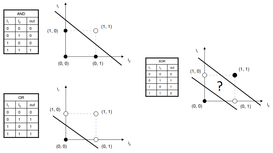
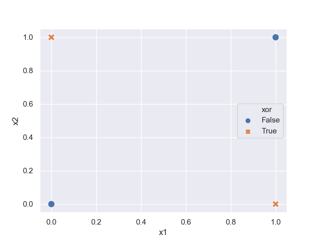
The XOR function is the simplest (afaik) non-linear function. Is is impossible to separate True results from the False results using a linear function.

def xor(x1, x2):
    """returns XOR"""
    return bool(x1) != bool(x2)

x = np.array([[0,0],[0,1],[1,0],[1,1]])
y = np.array([xor(*x) for x in inputs])

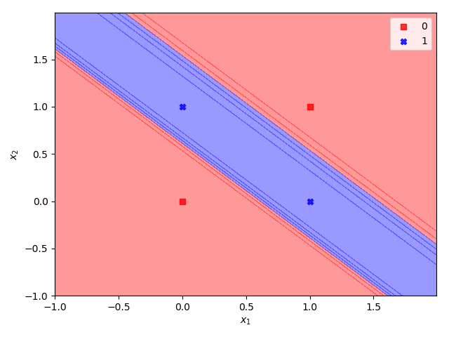
This is clear on a plot

import pandas as pd
import seaborn as sns
sns.set()

data = pd.DataFrame(x, columns=['x1', 'x2'])
data['xor'] = y
sns.scatterplot(data=data, x='x1', y='x2', style='xor', hue='xor', s=100)
No straight line (plane) can entirely separate all the True values from the False values.

A neural network is essentially a series of hyperplanes (a plane in N dimensions) that group / separate regions in the target hyperplane.

Two lines is all it would take to separate the True values from the False values in the XOR gate.

The Perceptron

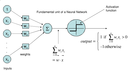
There’s lots of good articles about perceptrons. To quickly summarise, a perceptron is essentially a method of separating a manifold with a hyperplane. This is just drawing a straight line to separate an n-dimensional space into two regions: True or False. I will interchangeably refer to these as neurons or perceptrons. Arguablly different, they are basically the same thing.

A perceptron model from stackexchange

Activation functions

The way our brains work is like a sort of step function. Neurons fires a 1 if there is enough build up of voltage else it doesn’t fire (i.e a zero). We aim, via the percepton, to recreate this behaviour.

The problem with a step function is that they are discontinuous. This creates problems with the practicality of the mathematics (talk to any derivatives trader about the problems in hedging barrier options at the money). Thus we tend to use a smooth functions, the sigmoid, which is infinitely differentiable, allowing us to easily do calculus with our model.

def sigmoid(x):
    return 1/(1 + np.exp(-x))

Hyperplanes

A single perceptron, therefore, cannot separate our XOR gate because it can only draw one straight line.

How do we draw two straight lines? (from Kevin Swingler via Lucas Araújo)

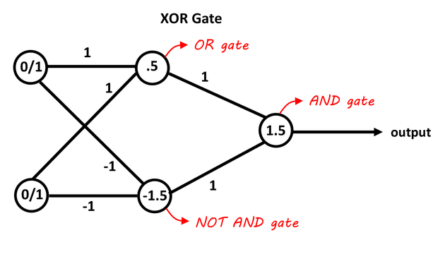
The trick is to realise that we can just logically stack two perceptrons. Two perceptrons that will draw straight lines, and another perceptron that serves to combine these two separate signals into a single signal that just has to differntiate between a single True / False boundary.

The XOR gate can be created by the following combination of a NOT AND gate and an OR gate (from blog.abhranil.net)

Learning parameters

The “knowledge” of a neural network is all contained in the learned parameters which are the weights and bias. The weights are multiplied to each signal sent by their respective perceptrons and the bias are added as $y(x) = wx + b$ where $w$ is the weight and $b$ is the bias.

The backpropagation algorithm (backprop.) is the key method by which we seqeuntially adjust the weights by backpropagating the errors from the final output neuron.

We define define the error as anything that will decrease as we approach the target distribution. Let $E$ be the error function given by

\[E = \frac{1}{2}(y - y_{o})^2\]

where $y_o$ is the result of the output layer (the prediction) and $y$ is the true value given in the training data.

Later we will require the derivative of this function so we can add in a factor of 0.5 which simplifies the derivative.

def error(target, prediction):
    return .5 * (target - prediction)**2
*Note: Explicitly we should define as the norm like, $E = \frac{1}{2}   y - y_{o}   ^2$ since $y$ and $y_{o}$ are vectors but practically it makes no difference and so I prefer to keep it simple for this tutorial.*

Algorithm

The learning algorithm consists of the following steps:

  1. Randomly initialise bias and weights
  2. Iterate the training data
    • Forward propagate: Calculate the neural net the output
    • Compute a “loss function”
    • Backwards propagate: Calculate the gradients with respect to the weights and bias
    • Adjust weights and bias by gradient descent
  3. Exit when error is minimised to some criteria

Note that here we are trying to replicate the exact functional form of the input data. This is not probabilistic data so we do not need a train / validation / test split as overtraining here is actually the aim.

Back propagation

We want to find the minimum loss given a set of parameters (the weights and biases). Recalling some AS level maths, we can find the minima of a function by minimising the gradient (each minima has zero gradient). Also luckily for us, this problem has no local minima so we don’t need to do any funny business to guarantee convergence.

Real world problems require stochastic gradient descents which “jump about” as they descend giving them the ability to find the global minima given a long enough time.

We therefore have several quantitites that require calculation

$\frac{\partial E}{\partial w_{o}}$,

$\frac{\partial E}{\partial w_{h}}$,

$\frac{\partial E}{\partial b_{o}}$

and $\frac{\partial E}{\partial w_{h}}$ where $h$ and $o$ denote hidden and output layers and $E$ is the total error given by

\[\frac{1}{2}(y - y_{o})^2\]

Output layer gradient

Starting at the output layer, and by chain rule,

\[\frac{\partial E}{\partial w_{o}} = \frac{\partial E}{\partial y_{o}} \frac{\partial y_o}{\partial a_{o}} \frac{\partial a_o}{\partial w_{o}}\]

This is true because the output layer $y_o = \sigma(a_o)$ varies with respect to the activation $a_o = w_o \cdot y_h + b_o$ in the output layer. The activation in the output layer varies with respect to the weights of the output layer. Recall that this is a partial derivative so we hold the bias of the output layer and the hidden layer output as constants. We can calculate all these terms.

The derivative of the Error with respect to the output layer is just

\[\frac{\partial E}{\partial y_{o}} = -(y - y_o)\]

due to the sneaky extra half

def error_derivative(target, prediction):
    return - target + prediction

The derivative of the output layer with respect to the sigmoid is

\[\frac{\partial y_o}{\partial a_{o}} = \frac{\partial \sigma(a_o)}{\partial a_o} = \sigma(a_o) (1 - \sigma(a_o)) = y_o (1 - y_o)\]
def sigmoid_derivative(sigmoid_result):
    return sigmoid_result * (1 - sigmoid_result)

The derivative of the activation function with respect to the weights is

\[\frac{\partial a_o}{\partial w_{o}} = y_h\]

which is just the result from the hidden layer.

The same is true for the bias (changing $w_o$ for $b_o$) except

\[\frac{\partial a_o}{\partial b_{o}} = 1\]

Hidden layer gradient

For the hidden layer we just keep expanding. Instead of taking $y_h$ as a variable we now treat it as a function that varies with the output of the hidden layer. Thus instead of stopping at $\frac{\partial a_o}{\partial w_o}$ we must continue since $a_o = w_o \cdot y_h + b_o$ is a fuction of $y_h$ which is no longer a constant.

Recall, if we vary $w_h$, $y_h = \sigma(a_h)$ and further, $a_h = w_h \cdot x + b$ where $x$ is the input training data.

Starting at the output layer, and by chain rule,

\[\frac{\partial E}{\partial w_h} = \frac{\partial E}{\partial y_o} \frac{\partial y_o}{\partial a_o} \frac{\partial a_o}{\partial y_h} \frac{\partial y_h}{\partial a_h} \frac{\partial a_h}{\partial w_h}\]

the three extra derivatives we need to calculate are

\[\frac{\partial a_o}{\partial y_h} = w_o\]

then recall the derivative of the sigmoid from before

\[\frac{\partial y_h}{\partial a_h} = y_h (1 - y_h)\]

and finally

\[\frac{\partial a_h}{\partial w_h} = x\]

and again the bias are the same except $\frac{\partial a_h}{\partial b_h} = 1$

Parameter updates

Let all the parameters be defined in the vector $\theta = (w_o, w_h, b_o, b_h)$. Then they are all updated like

\[\theta \leftarrow \theta - \alpha \frac{\partial E}{\partial \theta}\]

where $\alpha$ is the learning rate that is fixed at some constant (mysteriously, usually about 0.02) and this defines how fast we descend the gradient. Too fast and we overshoot and too small and it takes too long.

Explicitly for $w_o, b_o$ this would be,

\[w_o \leftarrow w_o + \alpha y^T_h \left((y_o - y) y_o (1 - y_o)\right)\\ b_o \leftarrow b_o + \alpha (y_o - y) y_o (1 - y_o)\]

where the $y_h^T$ denotes the transpose of the vector $y_h$. I was a bit underhand in the maths to simplify, but as we will see there is some care required with transposing of dot products when multiplying the weights and layers.

Implementation

Initialisation

Initialise the weights and bias like

import numpy as np

def xor(x1, x2):
    return bool(x1) != bool(x2)

x = np.array([[0, 0], [0, 1], [1, 0], [1, 1]])
y = np.array([xor(*i) for i in x])

# I explicitly name these for clarity
n_neurons_input, n_neurons_hidden, n_neurons_output = 2, 2, 1

# if this confuses you draw out all the possible wasy to connect the
# first two neurons remembering that we have only connections between layers
# and not between neurons on the same layer
w_hidden = np.random.random(size=(n_neurons_input, n_neurons_hidden))
b_hidden = np.random.random(size=(1, n_neurons_hidden))

w_output = np.random.random(size=(n_neurons_hidden, n_neurons_output))
b_output = np.random.random(size=(1, n_neurons_output))

Forward Propagation

We now have a neural network (albeit a lousey one!) that can be used to make a prediction. To make a prediction we must cross multiply all the weights with the inputs of each respective layer, summing the result and adding bias to the sum.

The action of cross multiplying all combinations of two vectors and summing the result is just the dot product, so that a single forward propagation is given as

def sigmoid(x):
    return 1/(1 + np.exp(-x))

y_hidden = sigmoid(np.dot(x, w_hidden) + b_hidden)
y_output = sigmoid(np.dot(y_hidden, w_output) + b_output)

where y_output is now our estimation of the function from the neural network.

Back propagation

The back propagation is then done

def sigmoid_derivative(sigmoid_result):
    return sigmoid_result * (1 - sigmoid_result)

grad_output = (- y + y_output) * sigmoid_derivative(y_output)
grad_hidden = grad_output.dot(w_output.T) * sigmoid_derivative(y_hidden)

The updates require a little explanation of the cheats I did before in the theory section. The function, $a_o = w_o \cdot y_h + b_o$ is actually a vector equation so explicitly, $a_o = y_h^T w_o + b_o$ and similarly, $a_h = x^T w_h + b_h$ which gives some intuition why we need to do the transposes below

w_output -= alpha * y_hidden.T.dot(grad_output)
w_hidden -= alpha * x.T.dot(grad_hidden)

The biases we recall had a derivative of 1. In reality this is the identity, or a vector of 1s so it reduces to a simple sum of all elements in the vector

b_output -= alpha * np.sum(grad_output, axis=0, keepdims=True)
b_hidden -= alpha * np.sum(grad_hidden, axis=0, keepdims=True)

Iteration / Early Stopping

We want to stop after some number of iterations. Therefore in our loop we can do something like below to exit early. We should also store some of the variables and gradients to ensure convergence.

import itertools

errors = []
params = []
grads = []
while True:
    # forward prop

    # calculate mean error of all the errors for this epoch
    e = error(y, y_output).mean()
    if e < 1e-4:
        break

    # back prop

    # update parameters

    # record intermediate results the concatenate just flattens all the
    # matrixes and arrays out into a single "row"
    errors.append(e)
    grads.append(np.concatenate((grad_output.ravel(), grad_hidden.ravel())))
    params.append(np.concatenate((w_output.ravel(), b_output.ravel(),
                                  w_hidden.ravel(), b_hidden.ravel())))

Experiment

Full script

Putting it all together we have

import itertools
import numpy as np

np.random.seed(42) # this makes sure you get the same results as me

def xor(x1, x2):
    return bool(x1) != bool(x2)

def sigmoid(x):
    return 1 / (1 + np.exp(-x))

def sigmoid_derivative(sigmoid_result):
    return sigmoid_result * (1 - sigmoid_result)

def error(target, prediction):
    return .5 * (target - prediction)**2

def error_derivative(target, prediction):
    return - target + prediction

x = np.array([[0, 0], [0, 1], [1, 0], [1, 1]])
y = np.array([[xor(*i)] for i in x], dtype=int)

alpha = 0.02
n_neurons_input, n_neurons_hidden, n_neurons_output = 2, 2, 1

w_hidden = np.random.random(size=(n_neurons_input, n_neurons_hidden))
b_hidden = np.random.random(size=(1, n_neurons_hidden))

w_output = np.random.random(size=(n_neurons_hidden, n_neurons_output))
b_output = np.random.random(size=(1, n_neurons_output))

errors = []
params = []
grads = []
while True:
    # forward prop
    y_hidden = sigmoid(np.dot(x, w_hidden) + b_hidden)
    y_output = sigmoid(np.dot(y_hidden, w_output) + b_output)

    # calculate mean error of all the errors for this epoch
    e = error(y, y_output).mean()
    if e < 1e-4:
        break

    # back prop
    grad_output = error_derivative(y, y_output) * sigmoid_derivative(y_output)
    grad_hidden = grad_output.dot(w_output.T) * sigmoid_derivative(y_hidden)

    # update parameters
    w_output -= alpha * y_hidden.T.dot(grad_output)
    w_hidden -= alpha * x.T.dot(grad_hidden)

    b_output -= alpha * np.sum(grad_output)
    b_hidden -= alpha * np.sum(grad_hidden)

    # record intermediate results
    errors.append(e)
    grads.append(np.concatenate((grad_output.ravel(), grad_hidden.ravel())))
    params.append(np.concatenate((w_output.ravel(), b_output.ravel(),
                                  w_hidden.ravel(), b_hidden.ravel())))

This takes about a minute to run on my macbook. We can now use the model to approximate XOR

>>> def predict(x):
>>>     y_hidden = sigmoid(np.dot(x, w_hidden) + b_hidden)
>>>     return sigmoid(np.dot(y_hidden, w_output) + b_output)
>>> predict(x)
array([[0.01505756],
       [0.98652214],
       [0.98652109],
       [0.01448912]])

As we can see we’re in the order of $10^{-2}$ which makes sense as we minimise the square error to the order of $10^{-4}$.

If this was a real problem, we would save the weights and bias as these define the model.

Convergence checks

We should check the convergence for any neural network across the paramters.

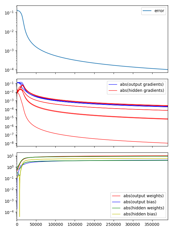
The simplest check is the error convergence. We should make sure that the error is decreasing. in larger networks the error can jump around quite erractically so often smoothing (e.g. EWMA) is used to see the decline.

It is also sensible to make sure that the parameters and gradients are cnoverging to sensible values. Furthermore, we would expect the gradients to all approach zero.

It is very important in large networks to address exploding parameters as they are a sign of a bug and can easily be missed to give spurious results.

I use Pandas combined with matplotlib to plot more easily

import matplotlib.pyplot as plt
import pandas as pd

fig, axes = plt.subplots(3, 1, figsize=(6, 8), sharex=True) 

pd.DataFrame(errors, columns=['error']).plot(ax=axes[0], logy=True)
df_grads = pd.DataFrame(grads)
df_params = pd.DataFrame(params)

for i in range(4):
    axes[1].plot(df_grads.iloc[:, i].abs(), c='b', label='abs(output gradients)' if i==1 else '__nolabel', lw=1)
for i in range(4, 12):
    axes[1].plot(df_grads.iloc[:, i].abs(), c='r', label='abs(hidden gradients)' if i==4 else '__nolabel', lw=1)

for i in range(1, 2):
    axes[2].plot(df_params.iloc[:, i].abs(), c='r', label='abs(output weights)' if i==1 else '__nolabel', lw=1)

axes[2].plot(df_params.iloc[:, 2].abs(), c='b', label='abs(output bias)', lw=1)

for i in range(3, 7):
    axes[2].plot(df_params.iloc[:, i].abs(), c='g', label='abs(hidden weights)' if i==3 else '__nolabel', lw=1)

for i in range(7, 9):
    axes[2].plot(df_params.iloc[:, i].abs(), c='y', label='abs(hidden bias)' if i==7 else '__nolabel', lw=1)

axes[1].legend()
axes[1].set_yscale('log')

axes[2].legend()
axes[2].set_yscale('log')

fig.tight_layout()
The convergence is smooth and decreasing which is ideal!

Vanishing gradient problem

It is noticable that the gradient of the hidden layer is considerably smaller than the output layer. This is normal.

In fact it presents a problem. One of the main problems historically with neural networks were that the gradients became too small too quickly as the network grew. In fact so small so quickly that the change in a deep parameter value causes such a small change in the output that it either gets lost in machine noise. Or, in the case of probabilistic models, lost in dataset noise.

This meant that neural networks couldn’t be used for a lot of the problems that required complex network architecture.

There are several workarounds for this problem which largely fall into architecture (e.g. ReLu) or algorithmic adjustments (e.g. greedy layer training).

The sigmoid, is a key offender in the mix. It maps input numbers onto a “small” range of [0, 1]. There are large regions of the input space which are mapped to an extremely small range. In these regions of the input space, even a large change will produce a small change in the output.

This notebook is an excellent example of choosing Relu instead of sigmoid to avoid the vanishing gradient problem.

Decision regions

We can plot the hyperplane separation of the decision boundaries. The sigmoid is a smooth function so there is no discontinuous boundary, rather we plot the transition from True into False.

This plot code is a bit more complex than the previous code samples but gives an extremely helpful insight into the workings of the neural network decision process for XOR.

import numpy as np
from matplotlib.colors import ListedColormap
import matplotlib.pyplot as plt

def predict(x):
    y_hidden = sigmoid(np.dot(x, w_hidden) + b_hidden)
    return sigmoid(np.dot(y_hidden, w_output) + b_output)

markers = ('s', 'X')
colors = ('red', 'blue')

x1_min, x1_max = x[:, 0].min() - 1, x[:, 0].max() + 1
x2_min, x2_max = x[:, 1].min() - 1, x[:, 1].max() + 1
xx1, xx2 = np.meshgrid(np.arange(x1_min, x1_max, resolution),
                       np.arange(x2_min, x2_max, resolution))

z = predict(np.array([xx1.ravel(), xx2.ravel()]).T)
z = z.reshape(xx1.shape)

fig, ax = plt.subplots()
ax.contourf(xx1, xx2, z, alpha=0.4, cmap=ListedColormap(colors))
ax.set_xlim(xx1.min(), xx1.max())
ax.set_ylim(xx2.min(), xx2.max())

for idx, cl in enumerate(np.unique(y)):
    ax.scatter(x=x[(y == cl).ravel(), 0],
               y=x[(y == cl).ravel(), 1],
               alpha=0.8, c=colors[idx],
               marker=markers[idx], label=cl)
ax.legend()
ax.set_xlabel('$x_1$')
ax.set_ylabel('$x_2$')
fig.tight_layout()

A converged result should have hyperplanes that separate the True and False values.

As you run the leanring process for longer, the decision boundary will approach the outer limit of the True region and towards inifinity will give the extremum of the True region (i.e. pass inifiniitely close to the inside of the squares)

References

Extracting Covid19 Data for NHS with Python

Contents

Lets assume you happen to stumble across the NHS data for Covid19 found at https://www.england.nhs.uk/statistics/statistical-work-areas/covid-19-daily-deaths/

Parse an Excel with Pandas

We can extract th dat for a funky plot like

import datetime
import pandas as pd

dt = datetime.date.today()
url_root = r'https://www.england.nhs.uk/statistics/wp-content/uploads/sites/2/2020/04/'
url_ts = url_root + f'COVID-19-total-announced-deaths-{dt.strftime("%-d-%B-%Y")}.xlsx'

_parser = lambda x: x in ['NHS England Region', 'Name'] or isinstance(x, datetime.datetime)
raw = pd.read_excel(url_ts, sheet_name=0, skiprows=15, usecols=_parser)
raw = raw.iloc[2:]
raw.index = pd.to_datetime(raw.index)

I opened the Excel file initially in Excel. There were 15 useless rows at the top. There was also an annoying column format where I only wanted dates, Name of hospital and NHS England Region. This is achieved by passing a function that will return True for any of these fields. There are also two junk rows athe the start of the dataframe and always convert date fields into datetime objects.

Cleaning Data

If you read the note in the excel file we see that numbers are rastically changed as and when the data comes in. This means that the last 5 days are highly variable. We want to separate this out and make it clear on any plot. Also the data is noisey. We can smooth with EWMA. I thought EWMA is a bit better than moving average because you get a continuous smoothing rather than a plot that jumps around as data moves in and out of the moving average window.

span = 10
unstable_region = 5
raw_diffs = raw.sum(axis=1).diff() # useful later
smoothed = raw_diffs.diff().ewm(span=span).mean()

stable = smoothed.iloc[:-unstable_region+1]
unstable = smoothed.iloc[-unstable_region:]

Plotting

This is pretty easy

import matplotlib.pyplot as plt
plt.ion()

fig, ax = plt.subplots()
stable.plot(title='Acceleration of Cumulative UK Deaths in NHS Hospitals',
            label='stable data',
            ax=ax) 
unstable.plot(ax=ax, color='red', ls='--', label='unstable data')

We can now plot the unstable dataset like

fig, ax = plt.subplots()
stable.plot(title='Acceleration of Cumulative UK Deaths in NHS Hospitals',
            label='stable data',
            ax=ax) 
unstable.plot(ax=ax, color='red', ls='--', label='unstable data')

ax.set_ylabel('change in daily fatalities')

Estimating Expected Updates

Now wehave the problem where the last 5 days of data are potentially garbage. WEe need to estimate somehow what the update might look like. That last few days of updates are available on the same landing page.

import requests
import bs4

# adjust the unstable data to take into account updated data
url_page = r'https://www.england.nhs.uk/statistics/statistical-work-areas/covid-19-daily-deaths/'
html = requests.get(url_page).content
soup = bs4.BeautifulSoup(
    html,
    "html.parser",
    parse_only=bs4.SoupStrainer('a')
)
url_updates = [
    l['href']
    for l in soup if 'xls' in l.get('href', '')
    and 'daily announced' in l.text.lower()
]

IN the above I parse the page for all a tags which are hyperlinks in HTML. Then I look for all hyperlinks that end in ".xls" and that also have the text "daily announced" in the link text.

Now I want to parse the date the update was given by. THis is a bit tricky because it’s clearly a human process as the files have slightly different names. We are at risk of the process breaking if someone changes the naming convention. I take the assumption "deaths" will always be the end of the file text name and be next to the date.

def get_offset_from_url(u):
    d = datetime.datetime.strptime(u[u.index('deaths-') + 7: u.index('-2020') + 5], '%d-%B-%Y')
    return (dt - d.date()).days

kws = dict(sheet_name='COVID19 daily deaths by age',
           skiprows=14, usecols=_parser, nrows=1)
updates_raw = pd.DataFrame(
    {
        get_offset_from_url(u): pd.read_excel(u, **kws).iloc[0]
        for u in url_updates
    }
)

I pass the data into a dataframe and read from the sheet name skipping useless rows and using the same column parser as before because we only want the dates and it doesn’t need to be recreated.

I’ll let you figure this next bit out, basically I’m recreating the data as it previously was.

updates_raw.columns.name = 'Adjustments n days ago'
updates_abs = updates_raw.copy()
updates_pct = updates_raw.copy()

all_cols = set(updates_raw.columns)
for i in reversed(sorted(updates_raw.columns)):
    # this is because of some errors in the data
    raw_as_of_date = (diff1 - updates_raw[all_cols].sum(axis=1))
    raw_as_of_date.iloc[-i-1:] = 0
    updates_pct[i] = updates_raw[i] / raw_as_of_date
    all_cols.remove(i)
    updates_abs[i] = updates_abs[i].shift(i)
    updates_pct[i] = updates_pct[i].shift(i)

updates_abs.index = pd.Index([(datetime.datetime.today() - i).days for i in updates_abs.index],
                         name='The date that was updated (n days ago)')
updates_pct.index = pd.Index([(datetime.datetime.today() - i).days for i in updates_pct.index],
                         name='The date that was updated (n days ago)')

There is a mistake in the dataset as well which I remove by raw_as_of_date.iloc[-i-1:] = 0. I add in the name parameters because I’m a bit OCD.

I then plot the data to make sure there isn’t any drastic change in the updates each day. What is possible is that in a stressed system there might be an increasing backlog.

fig2, (ax2, ax2b) = plt.subplots(2, sharex=True)
l = 0
colors = itertools.cycle(plt.rcParams['axes.prop_cycle'].by_key()['color'])
for col in updates_abs.iloc[-l:].columns:
    c = next(colors)
    (100*updates_pct.iloc[-l:][col].dropna()).plot(
        ax=ax2, lw=1, ls='--', color=c,
        label=f'update for previous days made {col} days ago'
    )
    (updates_abs.iloc[-l:][col].dropna()).plot(ax=ax2b, lw=1, ls='--', color=c, label=None)

c = next(colors)
(100*(updates_pct.iloc[-l:].mean(axis=1)).dropna()).plot(ax=ax2, color=c, label='mean')
((updates_abs.iloc[-l:].mean(axis=1)).dropna()).plot(ax=ax2b, color=c, label=None)

fig2.suptitle('Percentage change in the daily figures')
ax2.set_title("percentage daily adjustments aren't drastically increasing day by day",
              fontsize=8)
ax2.set_ylabel('Percentage change')
ax2.legend(fontsize=8)
ax2b.set_ylabel('Absolute change')

AS it turns out this isn’t the case and the updates are roughly the same each day and there is only about a 10% increase after the 5th day so the NHS note is correct in saying the last 5 days are the unstable region.

Estimating the expected updates is just done by integrating under the curve to get the expected updates as a percentage.

raw_diffs_adj = raw_diffs.copy()
for i in range(unstable_region):
    raw_diffs_adj.iloc[-i] = (updates_pct.mean(axis=1) + 1).iloc[-unstable_region:-i].prod() * raw_diffs.iloc[-i]

The updated plot

We use the axis handle from the plot above and update for the new estimates of what we expect the data to show.

smoothed_adj = raw_diffs_adj.diff().ewm(span=span).mean()

stable_adj = smoothed_adj.iloc[:-unstable_region+1]
unstable_adj = smoothed_adj.iloc[-unstable_region:]

fig3, ax3 = plt.subplots()
raw_diffs.plot(title='Daily fatalities in NHS Hospitals',
               label='original data', ax=ax3)
raw_diffs_adj.iloc[-unstable_region:].plot(ax=ax3, color='green', ls='--',
                   label='expected future adjustments')
ax3.set_ylabel('Fatalities attributed to each date')
ax3.legend(loc='upper left')

unstable_adj.plot(ax=ax, color='green', ls='--',
              label='expected future adjustments')

Estimating Impact of Government Measures

We now want to annotate where the UK government introduced quarantine phases. I found the parameters for the offset of 13 days byreading a load of medical papers which showed it took 13 days from infection to fatality as the low end of the interquartile range. I assume this would be where we start to see effects really feeding back into the data.

We can add labels for where we expect the data to be affected by isolation like

d0 = datetime.datetime(2020, 3, 16)
d1 = datetime.datetime(2020, 3, 23)
d2 = d0 + datetime.timedelta(days=13)
d3 = d1 + datetime.timedelta(days=13)

ax.axvspan(d3, smoothed_adj.index[-1], color='darkred', alpha=0.3, lw=0,
           label='national isolation + 13 days')
ax.axvspan(d2, d3, color='darkorange', alpha=0.3, lw=0,
           label='blanket symptomatic isolation + 13 days')
ax.legend(loc='lower left', fontsize=8)

Layout is better with

fig.tight_layout()

Full Example Script

import datetime
import pandas as pd
import itertools
import bs4
import requests
from urllib.request import HTTPError

dt = datetime.date.today()
url_root = r'https://www.england.nhs.uk/statistics/wp-content/uploads/sites/2/2020/04/'
url_ts = url_root + f'COVID-19-total-announced-deaths-{dt.strftime("%-d-%B-%Y")}.xlsx'

_parser = lambda x: x in ['NHS England Region', 'Name'] or isinstance(x, datetime.datetime)
raw = pd.read_excel(url_ts, sheet_name=0, skiprows=15, usecols=_parser)
raw = raw.iloc[2:]

raw = raw.set_index(['NHS England Region', 'Name']).T.cumsum()
raw.index = pd.to_datetime(raw.index)

span = 10
unstable_region = 5
raw_diffs = raw.sum(axis=1).diff() # useful later
smoothed = raw_diffs.diff().ewm(span=span).mean()

stable = smoothed.iloc[:-unstable_region+1]
unstable = smoothed.iloc[-unstable_region:]

fig, ax = plt.subplots()
stable.plot(title='Acceleration of Cumulative UK Deaths in NHS Hospitals',
            label='stable data',
            ax=ax) 
unstable.plot(ax=ax, color='red', ls='--', label='unstable data')

ax.set_ylabel('change in daily fatalities')

# adjust the unstable data to take into account updated data
url_page = r'https://www.england.nhs.uk/statistics/statistical-work-areas/covid-19-daily-deaths/'
html = requests.get(url_page).content
soup = bs4.BeautifulSoup(
    html,
    "html.parser",
    parse_only=bs4.SoupStrainer('a')
)
url_updates = [
    l['href']
    for l in soup if 'xls' in l.get('href', '')
    and 'daily announced' in l.text.lower()
]

def get_offset_from_url(u):
    d = datetime.datetime.strptime(u[u.index('deaths-') + 7: u.index('-2020') + 5], '%d-%B-%Y')
    return (dt - d.date()).days

kws = dict(sheet_name='COVID19 daily deaths by age',
           skiprows=14, usecols=_parser, nrows=1)
updates_raw = pd.DataFrame(
    {
        get_offset_from_url(u): pd.read_excel(u, **kws).iloc[0]
        for u in url_updates
    }
)
updates_raw.columns.name = 'Adjustments n days ago'
updates_abs = updates_raw.copy()
updates_pct = updates_raw.copy()

all_cols = set(updates_raw.columns)
for i in reversed(sorted(updates_raw.columns)):
    # this is because of some errors in the data
    raw_as_of_date = (raw_diffs - updates_raw[all_cols].sum(axis=1))
    raw_as_of_date.iloc[-i-1:] = 0
    updates_pct[i] = updates_raw[i] / raw_as_of_date
    all_cols.remove(i)
    updates_abs[i] = updates_abs[i].shift(i)
    updates_pct[i] = updates_pct[i].shift(i)

updates_abs.index = pd.Index([(datetime.datetime.today() - i).days for i in updates_abs.index],
                         name='The date that was updated (n days ago)')
updates_pct.index = pd.Index([(datetime.datetime.today() - i).days for i in updates_pct.index],
                         name='The date that was updated (n days ago)')

# check that daily adjustment aren't drastically increasing
# ie. that we can use an average of the last few days without
# implicitly concealing some exponential growth

fig2, (ax2, ax2b) = plt.subplots(2, sharex=True)
l = 0
colors = itertools.cycle(plt.rcParams['axes.prop_cycle'].by_key()['color'])
for col in updates_abs.iloc[-l:].columns:
    c = next(colors)
    (100*updates_pct.iloc[-l:][col].dropna()).plot(
        ax=ax2, lw=1, ls='--', color=c,
        label=f'update for previous days made {col} days ago'
    )
    (updates_abs.iloc[-l:][col].dropna()).plot(ax=ax2b, lw=1, ls='--', color=c, label=None)

c = next(colors)
(100*(updates_pct.iloc[-l:].mean(axis=1)).dropna()).plot(ax=ax2, color=c, label='mean')
((updates_abs.iloc[-l:].mean(axis=1)).dropna()).plot(ax=ax2b, color=c, label=None)

fig2.suptitle('Percentage change in the daily figures')
ax2.set_title("percentage daily adjustments aren't drastically increasing day by day",
              fontsize=8)
ax2.set_ylabel('Percentage change')
ax2.legend(fontsize=8)
ax2b.set_ylabel('Absolute change')

# we only see about 10% increase to data that was more than 5 days ago
# therefore we can adjust accordingly
raw_diffs_adj = raw_diffs.copy()
for i in range(unstable_region):
    raw_diffs_adj.iloc[-i] = (updates_pct.mean(axis=1) + 1).iloc[-unstable_region:-i].prod() * raw_diffs.iloc[-i]

smoothed_adj = raw_diffs_adj.diff().ewm(span=span).mean()

stable_adj = smoothed_adj.iloc[:-unstable_region+1]
unstable_adj = smoothed_adj.iloc[-unstable_region:]

fig3, ax3 = plt.subplots()
raw_diffs.plot(title='Daily fatalities in NHS Hospitals',
               label='original data', ax=ax3)
raw_diffs_adj.iloc[-unstable_region-1:].plot(ax=ax3, color='red', ls='--',
                   label='taking into account expected future adjustments')
ax3.set_ylabel('Fatalities attributed to each date')
ax3.legend(loc='upper left')

unstable_adj.plot(ax=ax, color='green', ls='--',
              label='expected future adjustments')

d0 = datetime.datetime(2020, 3, 16)
d1 = datetime.datetime(2020, 3, 23)
d2 = d0 + datetime.timedelta(days=13)
d3 = d1 + datetime.timedelta(days=13)

ax.axvspan(d3, smoothed_adj.index[-1], color='darkred', alpha=0.3, lw=0,
           label='national isolation + 13 days')
ax.axvspan(d2, d3, color='darkorange', alpha=0.3, lw=0,
           label='blanket symptomatic isolation + 13 days')
ax.legend(loc='lower left', fontsize=8)
fig.tight_layout()

11: Classes and Modules

Learning Outcomes

  • Be able to create a basic class
  • Interact with a class object
  • Understand the utility of classes
  • An idea of good and bad class usage
  • Be able to create modular code
  • Import from modular code

Contents

Classes 

Without necessarily knowing it you have been itnertacting with classes during this entire tutorial. That be said what is a class?


class Dog:
    """
    Creates a Dog. Note that you will normally not document __init__ but instead
    put then documentation under the ``class`` definition
    
    Args:
        name: The dogs name
        color: give a color
        speed: Give the top speed in mph. Must be >= 0
        weight: Give the weight in kg. Must be >= 0
    
    Example:
        >>> Dog('rover', 'brown', 10, 50)
    """
    def __init__(self, name, color, max_speed, weight):
        self.name = name
        self.color = color
        self.max_speed = max_speed
        self.weight = weight
        
        if max_speed <= 0:
            raise ValueError('Cannot have max_speed <= 0')
        if weight <= 0:
            raise ValueError('Cannot have weight <= 0')

    def noise(self):
        """
        Makes the noise of a dog
        
        Example:
            >>> Dog('ronald', 'green', 10, 50).noise()
            'woof'
        """
        return 'woof'

A class is an abstraction of the logic that defines something. In this instance ‘something’ is a Dog - or rather a pretty basic dog. Currently all our dog can do is Woof!

The __init__ method is used to define what arguments a class can take at it’s creation. We can similarly define a class like

class DogBase:

    def noise(self):
        return 'woof'

Style Tip Always define classes in ThisFormatOfText

but the we cannot specify any defining characteristics about DogBase so it kind of loses it’s individual charm - there are cases where DogBase would be increadibly useful but we won’t touch on those at this level.

What is self in a class

Functions within classes are known as class methods. This new namenclature kind of gives us a hint at a few things…

I can define a function outside of the class which doesn’t overwrite the function inside the class

>>> def noise()
...     return 'roar'
>>> Dog('ronald', 'purple', 10, 50).noise()
'woof'

Why is it called self?

Secondly, notice that all my class methods contain the variable name self as the first argument whereas my function did not have this requirement.

self is actually not required to be called self. In fact I could call it any name. It’s the same as using m for mass in Newton’s law F = m * a. I could easily replace Newton’s law with g = p * j and state that g is force, p is mass and j is acceleration.

The reason we use self is because it’s refers to the class object itself

What does self do?

Lets create an instance of Dog

>>> rover = Dog('rover', 'brown', 15, 50)

When we call

>>> rover.noise()

what happens internally is actually

>>> Dog.noise(rover)

thus self becomes rover!

Interacting with class attributes

Anything that is assigned to self becomes an attribute that we can interact with. This is another very useful property of a class: For storing intermediate results.

class Demo:
    """
    A demo taking in 3 integers, x, y, z

    Example:
        >>> d = Demo(1, 2, 3)
        >>> (d.x == 1) & (d.y == 2) & (d.z == 3)
        True
    """
    def __init__(self, x, y, z):
        self.x = x
        self.y = y
        self.z = z

    def method(self, a, b):
        """
        Calculates ``(x^y + z) * a * b``

        Example:
            >>> x, y, z, a, b = 1, 5, 76, 89, 2
            >>> d = Demo(x, y, z)
            >>> d.method(a, b) - (x**y + z) * a * b  < 1e-6
            True

            We can also extract the temporary reuslt afterwards
            >>> d.tmp - (x**y + z) < 1e-6
            True

            and we also stored the result
            >>> d.res - (x**y + z) * a * b  < 1e-6
            True
        """
        self.tmp = self.x**self.y + self.z
        self.res = self.tmp * a * b
        return self.res

Testing Tip As a side note I actually got the variable names on this really simple function wrong several times simply because I decided to rename them all! THe doctests saved me actually putting up incorrect code.

When to use Classes

This is all great but you don’t work in a Game Studio. This is geared towards banking so why do we care about Dogs?! We don’t, so lets start looking at trading strategies.

Just as a heasd up: This has no relation to how Nomura QIS calculate momentum. This is just a simple demonstration to how we would want to utilise classes for signals

Start with ideas as snippets then functions

The best way to start is normally with functions or single lines of code. As you become comfortable with components move then into functions.

Consider a simple momentum trading strategy: Simply define the momentum signal as the average of the sign of the return the n previous days

import numpy as np

def momentum_signal(s):
    """
    A simple momentum signal
    
    Args:
        s: A numpy array of some underlying instrument price
    
    Example:
        We expect the returns to be calculated like
        
        >>> import numpy as np
        >>> s = np.array([1. , 1.5, 1. , 1.5])
        >>> rets_expected = np.array([1.5/1-1, 1/1.5-1, 1.5/1-1])
        
        Then we take the sign of these returns which gives
        
        >>> np.sign(rets_expected)
        array([ 1., -1.,  1.])
        
        Finally we average the sign like
        >>> expected = np.sign(rets_expected).sum() / 3.
        
        and we can compare against our function using `np.allclose`
        because sometimes the values may vary ever so slightly due to machine
        precision

        >>> result = momentum_signal(s)
        >>> np.allclose(result, expected)
        True
    """
    if not isinstance(s, np.ndarray):
        s = np.array(s)         # we need it to be a numpy array for efficiency
    rets = s[1:] / s[:-1] - 1   # See exercise 11.2 to understand this
    return np.sign(rets).mean()

This function is pretty generic bcause it will just give the signal on whatever prices you send into it. However, you need logic to take the last n prices from a larger timeseries and may want to do this in a rolling process so as to create a backtest.

These two conditions generate the need for a class

When to avoid classes

As a beginner classes will almost always make debugging more complicated if you dive into them head first.

Remember that abstraction is a tool: You should only use tools if they make your work more productive.

An analogy is laying a drainage ditch in your back garden. An automated drainage ditcher is clearly far more adept at this task. By the time you source one and finally figure out how it works you could have already been at the pub. Also in using this new tool, it’s likely that you may misconfigure it and have a lot of issues as a result! Pick the right tool for the right job!

Example: A bad class

I regularly see code from beginners that will define a single class in a module that will never change in its parameterisation and will only ever be called once with functions that do indepedent tasks.

However, just because they functions were all for the specific task they may have wrote a class like

from yourfirms_quantlib import core

class TradeThingyForReportX:
    """
    The report I was asked to automate yesterday for that client
    
    Args:
        my_trades: A list of trade id numbers

    Example:
        >>> report = TradeThingyForReportX([432346, 3546457, 345324])
        >>> report.my_trades
        [432346, 3546457, 345324]
    """
    def __init__(self, my_trades):
        self.my_trades = my_trades
   
    def value_trades_usd(self):
        """Loads trades from some central db and values them in USD
        
        Example:
            >>> report = TradeThingyForReportX([432346, 3546457, 345324])
            >>> report.value_trades_usd()
            2389456.34
        """
        return core.PresentValue(self.my_trades)
    
    def rebuild_forward_curves_with_new_data(self, new_data):
        """Loads trades from some central db and values them in USD

        Args:
            new_data: A list of some kind of new params for the trades

        Example:
            >>> report = TradeThingyForReportX([432346, 3546457, 345324])
            >>> report.rebuild_forward_curves_with_new_data([{'start_date': 1}])
            
            Lets assume we can check in the core quantlib if they are mutated
            >>> core.trade_start_date_shock([432346, 3546457, 345324])
            [1, 1, 1]
        """
        # ...
        # some manipulation to reformat new_data
        # ...

        # assume this changes the IDs in memory during this python session
        # althought this would probabaly be a terrible idea in reality!
        core.rebuild_forward_curves(my_trades, new_data)


    def get_present_value_with_new_data(new_data):
        """
        Gets the PV for a report X with some scenario modifications

        Args:
            new_data: A list of some kind of new params for the trades

        Example:
            Lets assume our new_data allows us to bump parameters then

            >>> report = TradeThingyForReportX([432346, 3546457, 345324])
            >>> report.get_present_value_with_new_data([{'start_date': 1}])
            92309.6
        """
        self.rebuild_forward_curves_with_new_data(new_data)
        return self.value_trades()

Given that this report will never be used outside of this junior’s function: I would say that this is a bad example of writing a class.

Example: Avoiding bad classes

Instead I would write the above example as below which results in far less complexity and less code

from yourfirms_quantlib import core

def rebuild_forward_curves_with_new_data(my_trades, new_data):
    """Loads trades from some central db and values them in USD

    Args:
        my_trades: A list of trade id numbers
        new_data: A list of some kind of new params for the trades

    Example:
        >>> rebuild_forward_curves_with_new_data([7878676], [{'end_date': -1}])

        Lets assume we can check in the core quantlib if they are mutated
        >>> core.trade_end_date_shock([7878676])
        [-1]
    """
    # ...
    # some manipulation to reformat new_data
    # ...

    # assume this changes the IDs in memory during this python session
    # althought this would probabaly be a terrible idea in reality!
    core.rebuild_forward_curves(my_trades, new_data)


def pv_for_report_x(my_trades, new_data):
    """
    Gets the PV for a report X with some scenario modifications
    
    Args:
        my_trades: A list of trade id numbers
        new_data: A list of some kind of new params for the trades
    
    Example:
        Lets assume our new_data allows us to bump parameters then

        >>> pv_for_report_x([432346, 3546457, 345324], [{'start_date': 1}])
        92309.6
    """
    rebuild_forward_curves_with_new_data(my_trades, new_data)
    return core.PresentValue(my_trades)

When to move into a class

In my opinion there are two good reasonas to use classes in python

  1. You want to create many parameterisations of the same underlying logic (e.g. The Dog example)
  2. You have many functions that are constantly passing around the same objects

A class for our backtesting

Lets create an engine that can give us the signal at any given historic timepoint for our momentum strategy

Use pandas for timeseries analysis!

Doing timeseries analysis without using pandas is asking for trouble unless you’re an advanced programmer.

This is because pandas contains an index which travels with the arrays that prevents you tying youeslf in knots. A single bad index can and will totally breakdown any systemmatic signal.

Therefore let us start the creation of our strategy using a pandas Series (a pd.Series is just a single column of a pd.DataFrame) check this by creating df = pd.DataFrame({'a': [5, 6, 10]}) and selecting the column 'a' like df['a']

Writing the base logic

The following incorporates the basic framework in which we want to operate

class SimpleMom:
    """
    A simple momentum strategy
    
    Args:
        ts: The prices as a pandas DataFrame
        lookback: How many previous days we wish to create a signal from
    """
    def __init__(self, prices, lookback):
        if not isinstance(prices, pd.Series):
            raise ValueError('prices must be a pandas Series because we only want one column!')

        self.prices = pd.DataFrame(prices)
        self.lookback = lookback

Now lets add the signals in! This time we want to actually get the signal for a specific historical time point so we need some kind of reference to the time in the dataframe index

class SimpleMom:
    """
    A simple momentum strategy
    
    Args:
        ts: The prices as a pandas DataFrame
        lookback: How many previous days we wish to create a signal from

    Example:
        >>> import pandas as pd
        >>> prices = pd.Series([1. , 1.5, 1. , 1.5, 3.0])
        >>> sm = SimpleMom(prices, 3)
    """
    def __init__(self, prices, lookback):
        if not isinstance(prices, pd.Series):
            raise ValueError('prices must be a pandas Series because we only want one column!')

        self.prices = prices
        self.lookback = lookback

    def signal(self, t):
        """
        Gives the signal that we can observe at time ``t``
        
        Example:
            >>> sig = SimpleMom(pd.Series([1. , 1.5, 1. , 1.5, 4.0]), 3).signal(3)
            >>> np.allclose(1/3., sig)
            True
        """
        # this gives us all the prices up to but not including t
        # which is what we want because we can't observe the price at t
        # Think about EOD prices as an example... We can't see EOD for t
        # when are in day t
        prices_lookback = self.prices.loc[t - self.lookback: t]
        return momentum_signal(prices_lookback)

Modular Python

At this stage I would strongly recommend turning on autoreload in ipython which can be done like

In [0]: %load_ext autoreload

In [1]: %autoreload 2

This will allow your code to autoreload the changes as you edit them!

Example: Create a basic module

Create python files with the terminal in new directory called nnet the same directory like

./nnet/
    __init__.py
    core.py

This module will contain the generic mathematical building blocks required for a neural network. Our main module model.py will bring all of these components together to make a model.

Inside core.py put the following contents.

import numpy as np


def sigmoid(x):
    """
    The sigmoid function
    
    Example:
    
        This example shows how you can skip doctests
        on certain examples e.g. plots that are purely for
        demonstration and won't result in testable results

        >>> from nnet import core
        >>> import matplotlib.pyplot as plt  # doctest: skip
        >>> x = np.linspace(-10, 10, 100)    # doctest: skip
        >>> plt.plot(x, core.sigmoid(x))     # doctest: skip
        >>> plt.show()                       # doctest: skip
    """
    return 1 / (1 + np.exp(-x))

def forward_prop(x, w, b):
    """
    Forwards propagation
    
    Example:
        >>> import numpy as np
        >>> from nnet import core
        >>> x = np.array([[0],   # demonstrate that x is a column array
        ...               [1]])  # so has shape of (2, 1) - (rows, columns)
        >>> w = np.array([[.5, .5],
        ...               [.5, .5]])
        >>> b = np.array([[1], [1]])  # b is also a column array but on one line
        >>> core.forward_prop(x, w, b)
        array([[1.5],
               [1.5]])
    """
    # note that you can chain logic like below in python!
    if not (x.shape[0] == b.shape[0] == w.shape[-1]):
        raise ValueError('You have w, x, b wrong way round! '
                         f'Shapes: x: {x.shape}, w: {x.shape}, b: {b.shape}')
    return sigmoid(np.dot(w, x) + b)

__init__.py should be a blank file with no contents.

Example: Importing a Module

Now cd in ipython or the terminal so that nnet is a subdirectory. You will now be able to import the nnet module and use core.sigmoid as shown in the documentation example!

If you want to be able to import like

>>> import nnet
>>> nnet.core.sigmoid(1)
0.5

you will also need to alter the __init__.py to the following

from . import core

Example: Referencing other local modules

Create a new file model.py so that your directory looks like

./nnet/
    __init__.py
    core.py
    model.py

Inside model.py put the following

import numpy as np

from . import core


def predict(x, w0, w1, b0, b1):
    """
    Returns the prediction of a neural network
    using specified weights and bias

    Example:
        >>> import numpy as np
        >>> from nnet import model
        >>> x0, x1 = 1, 0
        >>> x = np.array([[x0], [x1]])
        >>> w0 = np.array([[.5, .5], [.5, .5]])
        >>> w1 = np.array([[.5, .5], [.5, .5]])
        >>> b0 = np.array([[.25], [.25]])
        >>> b1 = np.array([[1], [1]])
        >>> model.predict(x, w0, w1, b0, b1).round(3)  # rounding avoids floating point issues
        array([[0.843],
               [0.843]])
    """
    assert all((isinstance(o, np.ndarray) for o in (x, w0, w1, b0, b1)))
    layer1 = core.forward_prop(x, w0, b0)
    return core.forward_prop(layer1, w1, b1)

Style Tip Leave to blank lines after imports. Leave one blank line between libraries installed by default (import numpy as np at the top) and your own created modules (from . import core below)

You will now similarly be able to import and call predict as in the example if your present working directory has nnet as a subdirectory.

You can check your present working directory by typing pwd into ipython and check to see if nnet is a subdirectory by doing ls nnet either in ipython or the terminal

As an aside it should be slightly clearly why my bias for ipython is so strong

Aside: How Python installs libraries

You have effectively created a mini-library here on-the-fly. This is infact not too far off how libs are installed when you install a library in the terminal / powershell prompt like

$ python -m pip install SomeLibrary

What actually happens under-the-hood is that a system environment variable namd PYTHONPATH (similar to PATH) contains a list of all directories that python expects a python module (like you have created) to sit within as a subdirectory. These directories then behave as if your ipython terminal had them as the present working directory all at the same time.

As a hack you can see this working by doing

>>> import sys
>>> sys.path.append('/directory/that/containsnnet')

Then even if you are not in the correct directory, you will still be able to import nnet. This can be quite useful during development. Just as a heads up - never put this in finished python modules as it is awefully hacky and a terrible idea in general!

Exercises

Exercise 11.1: Understand your self

Modify the noise so that the dog now speaks english. You should include these two doctests in the Examples and make sure you can pass them

I have started this off for you as below. Note that you will need to rewrite the class method in Dog with the below function so it will need to be indented and underneath the definition of Dog

def noise():
    """
    Returns the noise of a fairly smart dog
    
    Example:
        >>> Dog('Rover', 'brown', 15, 50).noise()
        'I am Rover the Dog. I am brown. Woof!'
    
        >>> Dog('Sally', 'green', 15, 50).noise()
        'I am Sally the Dog. I am green. Woof!'
    """
    return

# Solve Me!

Exercises 11.2: Fixing indexing errors

In the example where we create SimpleMom there is actually a major bug.

See what happens if you make the t smaller than the lookback: In otherwords see what happens if you try and get a signal where there aren’t enough historic prices available for the required lookback

To further elaborate: If you have 4 prices in total as your history, you want to calculate the signal at day 2 but with a lookback window of 4 days… what happens!?

Propose a fix to this!

# Solve Me!

Next Topic

That’s it that’s all - Now go roam the wild ! At this stage you should be fairly proficient at beginner concepts. The best way to progress is to find a project idea to implement. Aim small with a very well defined success criteria. This is important because you want an end point at which you can determine you have succeeded and move on. It is also important to find something that you genuinely find interesting as a first project idea.

Migrating an Excel spreadsheet to python may seem useful but it is inantely boring as hell. How about controlling a toy drone? Scraping holiday websites for cheap deals? Silly fun ideas are by far the best ideas.

You are now truly a master of computers so go and have some realy fun!

10: Dictionaries and Sets

Learning Outcomes

  • How to use dictionary / set objects and differences to list / tuple
  • How to access dictionary objects in iteration
  • Utility of dictionaries as hashmaps
  • Utility of sets in dimensionality reduction

Contents

Sets

Sets only contain unique items

>>> trade_ids = [12342, 324562, 12342, 36452, 54767]
>>> set(trade_ids)
{12342, 36452, 54767, 324562}

We can also iterate a set like:

>>> for i in trade_ids:
...     print(i, end=',')
12342,324562,12342,36452,54767,

Set differences

They are also denoted by braces {}. Sets are a mathematical construct and python also supports some set logic such as set differences

>>> trade_ids_expected = {12342, 36452, 54767, 324569}  # shorter way of defining sets
>>> unexpected_trade_ids = set(trade_ids) - trade_ids_expected
>>> unexpected_trade_ids
{324562}

we can also do it the other way round to look for missing trades

>>> missing_trade_ids = trade_ids_expected - set(trade_ids)
>>> missing_trade_ids
{324569}

These two operations can be particularly useful when validating the inputs to functions.

Sets items must be immutable

We can also iterate sets in the same way that we iterate lists and tuples. Objects can also be part of sets as long as they are immutable - i.e. unchanging. Recall that lists are mutable and tuples are immutable.

This means that we can have a set of tuples

>>> set((1, 2,), (3, 4,))
{(1, 2,), (3, 4,)}

but not a set of lists

>>> {[1, 2], [3, 4]}
---------------------------------------------------------------------------

TypeError                                 Traceback (most recent call last)

<ipython-input-2-a0ff115cb325> in <module>()
----> 1 {[1, 2], [3, 4]}


TypeError: unhashable type: 'list'

Dictionaries

Dictionaries are python’s version of that is known as a hash map or hash table in other languages. If anyone in an interview asks you for a hash map in python you’ll know they just mean a dict (also they probably don’t really know python that well!)

All this jargon means is a key-value lookup where the key is unambigouously unique. Think VLOOKUP in Excel but if there couldn’t be any keys that are identical.

We set up a dictionary with a key value pair like follows

>>> d = {
...     'akey': 'avalue',
...     'anotherkey': 'avalue'
... }

values can be anything.

I actually wrote a load of stuff about this but I deleted it because I think you shoudl get used looking at python documentation now you are more familiar with the language.

See the offical python guide on dict - don’t bother with dict comprehensions yet as we will come onto those but have a read of the dictionaries and looping techniques sections.

Example: Trades by Asset Class

Lets assume we have the following data which we read in from a csv into a pandas DataFrame. Lets also assume that your credit and commodity desks for some reason give you the trade_id as a str - this is very annoying for you but a typical problem.

Finally, for any more advanced readers this example is focused on dict and not pandas so we shall avoid using pandas for now

>>> import pandas as pd
>>> data = [['rates', 346455, 568789.345],
...         ['rates', 3467457, 4568679.345],
...         ['rates', 56858, -6578965789.45],
...         ['fx', 93875, 67896789.34],
...         ['fx', 34896, -3464754.456],
...         ['fx', 30986, 0.3456457],
...         ['credit', '234537', 45765.456],
...         ['credit', '457568', -3455436.213],
...         ['credit', '3467457', 456546.034],
...         ['commodities', '93875', -34563456.23235],
...         ['commodities', '34457', 4560456.4567],
...         ['commodities', '457478', 4575678.345346],
...         ['equities', 3466, -457567.345],
...         ['equities', 564756, -12.93045],
...         ['equities', 457568, 546636.438996]]
>>> df = pd.DataFrame(data, columns=['risk', 'trade_id', 'dv01'])

How many trades are there per asset class with delta risk?

>>> trade_by_asset_class = dict()
>>> for asset_class, trade_id in df.values:
...     trade_by_asset_class[asset_class] = trade_id

Lets now figure out what went wrong here… Remembering the stack method we see that there are too many values to unpack and that the arrow is on the for line (if you are useing pyCharm - you know who you are - then you may have no arrow!)

With iteration errors it is often easiest to index the first element to see why we couldn’t unpack it:

>>> df.values[0]
array(['rates', 346455, 568789.345], dtype=object)

Here we can see there are three items and we are trying to unpack to two elements asset_class and trade_id therefore we need a third element even if we don’t currently care about the delta! A standard way of creating throwaway elements is to use _ like

>>> trade_by_asset_class = dict()
>>> for asset_class, trade_id, _ in df.values:
...     trade_by_asset_class[asset_class] = trade_id

but this doesn’t really help because each iteration we have overwritten the value!

>>> trade_by_asset_class
{'rates': 56858,
 'fx': 30986,
 'credit': '3467457',
 'commodities': '457478',
 'equities': 457568}

we therefore need to create a list as a value item and then append to the list - this is one of the most common dictionary structures.

>>> trade_by_asset_class = dict()
>>> for asset_class, trade_id, _ in df.values:
...     if asset_class not in trade_by_asset_class:
...         trade_by_asset_class[asset_class] = []
...     trade_by_asset_class[asset_class].append(trade_id)

Think about these operations if you have a large number of rows: The following should bve quicker have a think about why this might be the case…

>>> trade_by_asset_class = dict()
>>> for ac in set(df['risk']):
...     trade_by_asset_class[ac] = []
>>> for asset_class, trade_id, _ in df.values:
...     trade_by_asset_class[asset_class].append(trade_id)

which gives

>>> trade_by_asset_class
{'rates': [346455, 3467457, 56858],
 'fx': [93875, 34896, 30986],
 'commodities': ['93875', '34457', '457478'],
 'equities': [3466, 564756, 457568],
 'credit': ['234537', '457568', '3467457']}

we now have a structure for answering the question:

>>> for a, t in trade_by_asset_class.items():
...     print('risk: {:12s} trades: {:2d}'.format(a, len(t)))
risk: rates        trades:  3
risk: fx           trades:  3
risk: commodities  trades:  3
risk: equities     trades:  3
risk: credit       trades:  3

For more information string padding see: https://pyformat.info/#string_pad_align

Simplifying iterations with dictionaries

Lets imagine that the credit trading PnL system for some reason prepends '0s' on all the database ids under a length of 7 because some lunatic decided it looked nice in the 90s.

To link your PnL you will have to also prepend zeros to every trade_id

Whilst cussing out Diana Bloggs who retired last year after a distinguished trading career; but yet who also royally screwed you with one decision she made as a grad on a drizzly friday morning in 1999

We can zero pad integers to a length of 7 like

>>> str(346).zfill(8)
'00000346'

A naiive way of doing this would be just to call one of the following

>>> df['trade_id_pad'] = df['trade_id'].astype(str).str.zfill(8)

This example shows us two new operations: Firstly that we can call .astype on a pandas.Series (a series is a single column of a DataFrame). Secondly, if a pandas series is a str type then we can call .str to access operations that are normally found within str object types.

Imagine now that this dataframe is $10^6$x larger

WARNING if your laptop is aweful you may not want to run this next section

>>> df = pd.DataFrame(data*1e6, columns=['risk', 'trade_id', 'dv01'])

Timing this for me took about 10 seconds!

In [100]: %timeit df['trade_id'].astype(str).str.zfill(8)
10.5 s ± 464 ms per loop (mean ± std. dev. of 7 runs, 1 loop each)

Lets now simplify the process by using the hashmap

In [101]: %%timeit
     ...: trade_ids = df['trade_id'].unique()  # pandas way to get unique items is fast
     ...: lookup = {}
     ...: for trade_id in trade_ids:
     ...:     lookup = {trade_id: str(trade_id).zfill(8)}
     ...: df['trade_id_pad'] = df['trade_id'].apply(lookup.get)
     ...: 
2.38 s ± 28.1 ms per loop (mean ± std. dev. of 7 runs, 1 loop each)

Here we see the .apply method in action. This is pandas version of a map. A map iterates a single function across an array of items. map actually exists in python as a default function and we can call it like:

>>> list(map(str, [3456, 4576, 7343]))
['3456', '4576', '7343']

and

>>> list(map(len, ['36', '45sd76', '7343']))
[2, 6, 4]

pandas.Series.apply works in the same way and in this example iterates the .get method of lookup across every item in the dataframe.

Here the lookup method is exceedingly fast and creating it only requires us to use the far slower line str(trade_id).zfill(8) 15 times instead of 15 million times!

Exercises

Exercise 10.1: Dimensionality reduction

This example aims to build on previous examples to reinforce the idea of hash maps for reducing complexity.

You are working on an end-of-day regulatory risk model that requires the revaluation of all trades (e.g. Basel III: FRTB Sensitivities Based Approach).

You have been instructed to calculate the present value (PV) as a new column in an Excel sheet. Someone else has done this and complained it was impossibly long and took over 40 hours to calculate. They have requested access to a compute grid to speed up their Excel sheet worth $10k per year.

Assume your pricing function to get the PV of the trade is this:

>>> import time
>>> import numpy as np
>>> np.random.seed(42)
>>> def my_pricing_function(trade_id):
...     """Gets the given a trade_id and returns a random pv"""
...     time.sleep(.1)
...     return 2e9 * np.random.random() - 1e9

and it is called in Excel something like =MY_PRICING_FUNCTION($B3) where $B3 references the trade_id and is dragged down the column B for all 10000 rows.

Assume we have already read the Excel sheet with python and it gives us a dataframe like below

>>> import pandas as pd
>>> data = [['rates', 346455, 568789.345],
...         ['rates', 3467457, 4568679.345],
...         ['rates', 56858, -6578965789.45],
...         ['fx', 93875, 67896789.34],
...         ['fx', 34896, -3464754.456],
...         ['fx', 30986, 0.3456457],
...         ['credit', '234537', 45765.456],
...         ['credit', '457568', -3455436.213],
...         ['credit', '3467457', 456546.034],
...         ['commodities', '93875', -34563456.23235],
...         ['commodities', '34457', 4560456.4567],
...         ['commodities', '457478', 4575678.345346],
...         ['equities', 3466, -457567.345],
...         ['equities', 564756, -12.93045],
...         ['equities', 457568, 546636.438996]]
>>> df = pd.DataFrame(data * 10000, columns=['risk', 'trade_id', 'dv01'])

Currently this pricing function is being called like

>>> df['pv'] = df['trade_id'].apply(my_pricing_function)

Use your knowledge of dictionaries to reduce the problem set and claim a portion of the cost savings for your bonus.

# Solve me

Next Topic

11: Classes and Modules

09: Lists and Tuples

Learning Outcomes

  • Declare and use both list and tuple
  • Differences between list and tuple
  • Some list operations
  • Mutable vs. immutable types
  • numpy arrays
  • vector operations on numpy arrays

Contents

tuple types

A tuple consists of a number of values separated by commas, for instance:

>>> t = 12345, 54321, 'hello!'
>>> t[0]
12345
>>> t
(12345, 54321, 'hello!')

They may be nested

>>> u = t, (1, 2, 3, 4, 5)
>>> u
((12345, 54321, 'hello!'), (1, 2, 3, 4, 5))

As you see, on output tuples are always enclosed in parentheses, so that nested tuples are interpreted correctly; they may be input with or without surrounding parentheses

Note When you create a tuple of one item you must always include a trailing comma like

>>> (1,)
(1,)

else it doesn’t create a tuple

>>> (1)
1

empty tuples can be created without a comma

>>> ()
()

this is also the same with an empty list

Indexing

Access items by referring to the index number (starting from 0)

>>> t = 12345, 54321, 'hello!', 'goodbye!'
>>> t[1]
54321

Negative indices start from the back and in the reverse

>>> t[-1], t[-2], t[-3], t[-len(t)]
('goodbye!', 'hello!', 54321, 12345)

Note t[-0] == t[0] so the reverse indexing actually starts at 1

Ranges of indices can be specified by the function slice which specifies the slice from and including the start index to but not including the end index

>>> a_tuple = 0, 1, 2, 3, 4, 5, 6, 7,
>>> a_tuple[slice(0, 2)]
(0, 1)

An optional thirs argument (the step) can also be specified like

>>> a_tuple[slice(0, None, 2)]
(0, 2, 4, 6)

Here we gave a step of 2 so it starts at the 0th item and returns every 2nd index until the end.

In the slice object providing None gives the default behaviour which is to start at 0 and slice to the end with a step of 1… This is given by

>>> a_tuple[slice(None, None, None)]
(0, 1, 2, 3, 4, 5, 6, 7)

In reality no-one really uses slice as there is a shorthand for it: The colon :!

When used between square brackets as an indexing operation is effectively separates what would otherwise be a call to the slice1 operator for example

>>> a_tuple[3:]
(3, 4, 5, 6, 7)

remember slices are up until (NOT INCLUSIVE) of the end index

>>> a_tuple[-4:-1]
(4, 5, 6)

this is the same as slice(0, 5, 2)

>>> a_tuple[0:5:2]
(0, 2, 4)

this is the same as slice(1, None, 2)

>>> a_tuple[1::2]
(1, 3, 5, 7)
>>> a_tuple[::-2]  # same as slice(None, None, -2)
(7, 5, 3, 1)

A side note on range

We have used range a few times. It is worth pointing out that its arguments operate in exactly the same way as slice. Except, instead of returning an index slice, it returns actual index values as a special range object.

>>> a = range(5)
>>> for i in a:
...     print(i, end=', ')
0, 1, 2, 3, 4,
>>> a
range(0, 5)

This can be converted to a list or tuple if we wish to use it as such

>>> list(range(5)), tuple(range(6, 2, -1))
([0, 1, 2, 3, 4], (6, 5, 4, 3))

list types

A list is a collection which is ordered and changeable. In Python lists are written with square brackets.

>>> this_list = ["apple", "banana", "cherry"]
>>> this_list
['apple', 'banana', 'cherry']

Lists are indexed in eactly the same ways as tuples

>>> this_list[1::-1]
['banana', 'apple']

We have already encountered .append. There are also other additional things with lists as we have extra methods available, some are shown below

>>> fruits = ['pear', 'banana', 'kiwi', 'apple', 'banana', 'grape']
>>> fruits.index('banana', 4)  # Find next banana starting a position 4
4

if no argument is provided it will pop -1

>>> fruits.pop(0)
'pear'

pop will also remove that item from the list

>>> fruits
['banana', 'kiwi', 'apple', 'banana', 'grape']

Both list and tuple types can be multiplied

>>> fruits[:2] * 2
['banana', 'kiwi', 'banana', 'kiwi']
>>> [tuple(fruits[:2])] * 2
[('banana', 'kiwi'), ('banana', 'kiwi')]

For a more complete list google something like “list methods python”

Example: Fibonacci Series

Here we use use the slice notation and python’s builtin sum function to simplify

>>> result = [0, 1]
>>> for i in range(5):
...     result.append(sum(result[-2:]))
>>> result
[0, 1, 1, 2, 3, 5, 8]

Example: A common misunderstood feature with the python list

>>> a_list = list(range(3))
>>> b_list = [a_list] * 3
>>> a_list.append('test')
>>> b_list
[[0, 1, 2, 'test'], [0, 1, 2, 'test'], [0, 1, 2, 'test']]

Whereas with tuples…

>>> a_tuple = tuple(range(3))
>>> b_tuple = (a_tuple,) * 3
>>> a_tuple += ('test',)
>>> b_tuple
((0, 1, 2), (0, 1, 2), (0, 1, 2))

Mutable vs. Immutable object types

Though tuples may seem similar to lists, they are often used in different situations and for different purposes

  1. Immutable objects can’t be changed.
  2. Mutable objects can be changed.

Immuatable object types like tuples cannot be mutated by assignment

>>> example_tuple = 1, 2, 3, 4
>>> example_tuple[2] = 5

---------------------------------------------------------------------------

TypeError                                 Traceback (most recent call last)

<ipython-input-36-3faa60cab3a6> in <module>()
      1 example_tuple = 1, 2, 3, 4
----> 2 example_tuple[2] = 5


TypeError: 'tuple' object does not support item assignment

Mutable object types like lists can be mutated by assignment

>>> example_list = [1, 2, 3, 4]
>>> example_list[2] = 5
>>> example_list
[1, 2, 5, 4]

A brief foray into c

Python was concieved as a scriptiong language built on the more low level language c. In c, programmers must be more-so aware that variables are simply link to memory address locations (Ever heard of RAM?). The random access memory (RAM) is where all these variables are stored. Conceptually imagine it as a big list with numbers assigned to it

We can query what the address location of each python object is by doing

>>> id(0)    # always put comments at least 1 space away from the last code piece
>>> id([0])  # unless visually making a block like this
4532216456

From this we can see that the object 0 has an address location and the object [0] has another different address location

What a mutable type really means is that we can change the address location of the type’s contents

>>> example_list = list(range(5))  # remember that a range(n) give an iterable from 0 to n-1
>>> id(example_list), example_list
(4534667592, [0, 1, 2, 3, 4])

whilst keeping the memory address of the container the same

>>> example_list += [5]             # note that you can put any math operator infront of =
>>> id(example_list), example_list  # to do an inplace assignment! e.g. -=, /=, %= etc
(4534667592, [0, 1, 2, 3, 4, 5])

Whereas with the tuple

>>> example_tuple = tuple(range(5))
>>> id(example_tuple), id(example_tuple)
(4532001432, 4532001432)

the address changes when it is mutated

>>> example_tuple += (5,)
>>> id(example_tuple), example_tuple
(4531868968, (0, 1, 2, 3, 4, 5))

Important note about address locations

If the variable is assigned to another variable, the variable points to the same address location which can be seen by

>>> example_tuple = tuple(range(5))
>>> another_variable = example_tuple
>>> id(example_tuple), id(another_variable)
(4532001784, 4532001784)

However, if we then change the address location of the original variable we break the link!

>>> example_tuple += (5,)
>>> id(example_tuple), id(another_variable)
(4531868872, 4532001784)
>>> example_tuple, another_variable
((0, 1, 2, 3, 4, 5), (0, 1, 2, 3, 4))

Whereas with mutable types like lists this reference persists!

>>> example_list = list(range(5))
>>> another_variable = example_list
>>> example_list += (5,)
>>> id(example_list) == id(another_variable)
True

A better way of checking the variables are exactly the same object value is by using is

>>> example_list is another_variable
True

A slice, will create a copy of a list object to a new address location. A blank slice will also do this

>>> example_list[:] is another_variable
False

For a more detailed overview of how exactly this works check out https://realpython.com/pointers-in-python/#immutable-vs-mutable-objects

Numpy Arrays

Numpy arrays are exceeedingly important to your future career as a python expert! They offer a way of doing optimised mathematics on lists.

The need for numpy arrays

Take the following as an example:

>>> arr = list(range(3))

Note that we can’t simply multiply a normal list and expect its elements to be doubled! The example below is expected behavour.

>>> arr * 2
[[1, 2, 3], [1, 2, 3]]

Think of a list like an object e.g. like an apple. If you multiply 10xApples you don’t suddenly expect 10x the number of seeds and one apple. As with the 10 apples you should expect 10 lists.

Thus we are required to do something like

>>> arr2 = arr.copy()  # As a teaser, try without .copy() and see what happens to arr!
>>> for i in range(arr.shape[0]):
...     arr2[i] = arr[i] * 2

The numpy solution

Compare to the numpy solution

>>> import numpy as np
>>> arr = np.array([1, 2, 3])
>>> np.array(arr) * 2
array([0, 2, 4])

In fact we can use np.arange to further simplify

>>> np.arange(3) * 2

Not only is this more concise, but numpy uses optimised C++ libraries that are incredibly difficult for humans to beat in terms of speed. Thus all operations we can push to the C++ part of numpy are as fast if not faster than some seriously intense C++ code (As a reminder C++ is a very fast language and what most core quant pricers are written in as a result)

As an example you may have a look at this numpy module which does matrix multiplication (note matmul is actually arr * arr.T not arr * 2) this will call a library called BLAS if possible which is a highly optimised linear algebra module written in Fortran and C++. In a nutshell: Goodluck at writing faster code than the authors of BLAS routines.

Iteration and indexing in numpy

Iteration and indexing in numpy are somewhat funky and this can make newwer users veryu confused between list and numpy.array iteration… I will try to not confuse you by making explicit what is specifically only allowed in numpy and what is allowed in list objects as well

All normal list indexing tricks can be used on numpy arrays

>>> import numpy as np
>>> arr = np.arange(10)
>>> arr[::-1]
array([9, 8, 7, 6, 5, 4, 3, 2, 1, 0])
>>> arr[:9]
array([0, 1, 2, 3, 4, 5, 6, 7, 8])

Masking

However only in numpy arrays we can use an array itself to mask or select items

>>> arr[arr > 5]
array([6, 7, 8, 9])

This will not work in a normal python list!

>>> l = list(range(10))
>>> l[l > 5]
---------------------------------------------------------------------------
TypeError                                 Traceback (most recent call last)
<ipython-input-24-33f477ef3cbe> in <module>()
      1 l = list(range(10))
----> 2 l[l > 5]

TypeError: '>' not supported between instances of 'list' and 'int'

This works because solely because

>>> arr > 5
array([False, False, False, False, False, False,  True,  True, True, True])

as a comparison see what happens when we do

>>> arr[[True] * 3 + [False] * 7]
array([0, 1, 2])

similarly we could do (remember the bitwise logic?)

>>> arr[(arr == 2) | (arr == 5)]
array([2, 5])

Fancy indexing

Another thing we can do in numpy is index explicitly with another array

>>> arr = np.arange(10)**2
>>> idx = np.arange(10) * 3
>>> arr[idx[idx < 10]]  # take this statement apart to understand it!
array([ 0,  9, 36, 81])

Whereas a similar statement won’t work with lists

>>> l = list(range(10))
>>> l[[0, 2, 4]]
---------------------------------------------------------------------------
TypeError                                 Traceback (most recent call last)
<ipython-input-38-5efbb062c778> in <module>()
      1 l = list(range(10))
----> 2 l[[0, 2, 4]]

TypeError: list indices must be integers or slices, not list

Confusingly, we can actually use a raw list to index a numpy array in fact we can use both list and tuple

>>> arr = np.arange(10)**2
>>> l = [3, 7, 9]
>>> arr[l]
array([ 9, 49, 81])

Optimising code for numpy

The key takeaway is to push all our compute into numpy’s C++ core

How do we achieve this in practice?

It can be tricky but in short use numpy arrays where possible for any math that needs to be done on every element this includes ** + / - * % // ^ | & as examples.

>>> np.arange(100)

Exercises

Exercise 9.1: Nested loops

This exercise is to help you understand iteration across more than one dimension.

Find the trace of the matrix a. The trace is defined as the sum of all the diagonal elements (this is 14 from visual inspection).

a = np.array([[1, 3, 5],[1, 4, 6],[7, 6, 9]])
>>> a
array([[1, 3, 5],
       [1, 4, 6],
       [7, 6, 9]])

Hint You may also want to play with

>>> for i, ai in enumerate(a):
...     print(i, ai)

recalling how multiple variable assignment works. Google may be your friend here!

Hint For the less maths-inclined the diagonal is [1, 4, 9]. We don’t want the anti-diagonal of [5, 4, 7].

# Solve me!

Exercise 9.2: Monte Carlo modelling using Geometric Brownian Motion

This exercise is to expand on the previous example with a bit of quantitative finance (Don’t worry though the maths will all be solved out for you!).

Here you will be guided through a monte carlo stock price model using Geometric Brownian Motion. You will also show that the returns from a GBM model follow a normal distribution.

This exercise is intended to be partcularly challenging and may require some googling but don’t give up - 99% of coding is being frustrated and feeling stupid… I sort of didn’t tell you that when you signed up haha!

Exercise 9.2.1: Storing iteration results in a list

Modify your previous example to the brownian motion exercise so that you store the results in a list named path while the stock price is greater than 0. Set path_len = 504 (i.e. 2 years) and only run for this many time steps.

Use the same values for dt = 1/252, sigma, mean etc that you used before, some (not all) are shown below

import numpy as np

np.random.seed(42)
sigma = .6729                           # annualised volatility of 67.29%
dt = 1/252                              # using annualised vol so need days as frac of yr
r = 0.02                                # annualised expected return
path_len = 504                          # 2 years of 252 business days
# solve me

as a check you should get the following

>>> path[:5]
[100,
 102.04421752046065,
 101.36484570799986,
 104.10104255605592,
 110.95250573627207]

Exercise 9.2.2: Plotting results

Plot your stock path using matplotlib - you will certainly want to google this

Hint Just use plt.plot nothing fancy!

# Solve me!

you should get the following

Stonks!

Exercise 9.2.3: Monte Carlo

In Exercise 9.2.1 you simulated a single path of a stock using GBM. Now create paths_num = 1000 paths and store each of these paths in another list named paths

Hint paths will be a list of lists & you will require two for loops. I have declared the empty list for you to fill below and to help you on the way I have done the first loop… You will need to finish the code off by adding another loop and the formula for caluclating $s_t$.

Lets restrict this time to one year of simulation to save our CPUs.

import numpy as np

np.random.seed(42)
sigma = .6729                           # annualised volatility of 67.29%
dt = 1/252                              # using annualised vol so need days as frac of yr
r = 0.02                                # annualised expected return
path_len = 252                          # only simulating 1y this time

paths_n = 1000
paths = []
for i in range(paths_n):
    s_t = 100
    path = [s_t]
    ...
    # solve me!

(The full solution takes about 3-4seconds to run on my macbook) TO verify your solution you should get

>>> paths[3][:5]
[100,
 104.481881330148,
 100.2784519513296,
 112.02421958412168,
 114.29778249864029]

Exercise 9.2.4: Plotting multiple lines on one plot

Plot all 1000 paths with pandas using dt as the index. This is a little more involved so read carefully!

When we created paths we created an object like

[
    [ s_00, s_01, ... , s_0n],  # indexed by paths[0]
    [ s_10, s_11, ... , s_1n],  # indexed by paths[1]
    [ ... , ... , ... , ... ],
    [ s_m0, s_m1, ... , s_mn]   # indexed by paths[m]
] #   ^paths[m][0]      ^paths[m][n]

This makes the zeroth axis the path index and the first axis the time index. However, in pandas and plotting in matplotlib we generally store the time index as the zeroth index and the path index as the first index.

To store in pandas we need to transpose (swap round the referencing) so that in the above example we would change paths[m][n] -> paths[n][m]. This is the same as transposing in Excel.

You can do this with a few different options

  1. paths_df = pd.DataFrame(paths).T
  2. paths_df = pd.DataFrame(list(zip(*paths)))
  3. paths_df = pd.DataFrame(np.array(paths).T)

For sanity would should also probably make the index match the timesteps we are using. Lets create a proper index.

import pandas as pd
import numpy as np
index = pd.Index(np.arange(path_len) * dt, name='years')

Now create the DataFrame with this index. Google if you get stuck.

paths_df = pd.DataFrame(paths, columns=index).T

Make sure that you can pass this test! If you can’t think about the order in which you created the index and then transposed the DataFrame

assert all(paths_df.index.values == index.values)

Now plot with the default pandas plot function. Make sure to pass the argument legend=None!

# Solve me!

you should get the following

Lots of stonks!

Exercise 9.2.5: Prove empirically GBM returns are Normally distributed

Prove that the 1-step stock returns are normally distributed under the GBM model by fitting a Gaussian distribution to the probability distribution function of the 1-day returns - Don’t worry it’s not as hard as it sounds :)

Exercise 9.2.5.1: Calculate 1-day returns using a pandas object

You will need to calculate 1-day returns. You have two options for this:

  1. Absolute returns $\frac{s_{t} - s_{t-1}}{s_{t-1}}$
  2. Log returns $\ln s_{t} - \ln s_{t-1}$

Without proof 2 is equal to 1 if $\Delta t \ll T$

e.g. if using years you want to be using a unit of $\Delta t$ that is roughly 100th of a year or smaller

Hint there are four things that might help in googling: "pandas diff", numpy natural log, "pandas shift", "pandas dropna" also remember Google !!

rets_1d = ...
# Solve me!

You should get the following as a check

>>> rets_1d.iloc[:3, :2]
                 0         1
years                       
0.003968  0.020236  0.038088
0.007937 -0.006680  0.089136
0.011905  0.026636  0.042946

Exercise 9.2.5.3: Check your results

This isn’t so much of an exercise but simply a check for the previous exercise to ensure you have it correct! The maths isn’t too important. If you like, you can ignore it all and just run the code below. You should expect differences less than 1% if you have it correct

Without proof (see here for one) we state that the n-day returns, $R_n$ follow a Normal distribution

\[R_n \sim \mathcal{N}(\mu_n, \sigma_n)\]

where

\(\mu_n = \left(r_T - \frac{1}{2}\sigma_T^2\right)n\Delta t\) \(\sigma_n = \sigma_T \sqrt{n\Delta t}\)

such that for T=252 (i.e. a year in our model) $r_T$ is the annualised rate of return (drift) and similarly $\sigma_T$ is the annualised volatility.

Lets take as a fact that we can model a probability distribution function (how likely an event) by using scipy.stats.norm.fit. Then the following snippet of code will confirm your results with theory as a check

# rets_1d should be your result from previous ... you should be able to run it to get the below
import scipy.stats
mean_th = (r - .5*sigma**2)*dt
stdv_th = sigma * np.sqrt(dt)

mean_ac, stdv_ac = scipy.stats.norm.fit(rets_1d)
print(f'Difference in mean samples vs theory: {100*(mean_th - mean_ac)/mean_ac:5.2f}%')
print(f'Difference in stdv samples vs theory: {100*(stdv_th - stdv_ac)/stdv_ac:5.2f}%')

Note Google f-string formatting!

After running the code about you should get the following the show that you have converged to the mean and standard deviation of a normal distribution

Difference in mean samples vs theory:  0.99%
Difference in stdv samples vs theory: -0.01%

Exercise 9.2.5.3: Plot theory vs. empirical results (reusing matplotlib axes)

This exercise isn’t so much an exercise rather than an example of how to resuse a matplotlib axis object to draw another line.

Compare this with the theory visually by plotting the theoretical distribution and showing its equivalence with the following code

import scipy.stats

# you can access the numpy array beneath the pandas object by .values - then everything is numpy again
rets_1d_all_paths = rets_1d.values.ravel() # get the returns from every path for more samples (google ravel)
x = np.linspace(-.5, .5, 200)              # an array of 200 numbers equally spaced between -.5 and .5 

# note that you can chain "." methods in ()
# because recall that unless you have (item,) it doesn't create a tuple!
ax = (
    pd.Series(rets_1d_all_paths) # convert back to pd.Series to use .hist()
    .hist(bins=100, density=True, label='1-day Monte Carlo')
)

# use the same axis object that was returned from .hist() 
theory = scipy.stats.norm.pdf(x, mean_th, stdv_th)
ax.plot(x, theory, alpha=0.5, label='1-day Analytic')
ax.legend()

you should get the following

Standard!

[Optional: This requires undergrad maths!] Exercise 9.2.5.4: Show this holds for 20-day returns

Show the same is true for 20day returns by plotting the relationship with 20-day returns

Note that this exercise is really aimed at structurers, derivatives traders and quants - if you haven’t studied stochastic calculus at university then just ignore this question or ask a quant if you find it interesting

# Solve me!

you should get the following

Someone sat on this one

Next Topic

10: Dictionaries and Sets

08: Functions and Editors

Learning Outcomes

  • Declare a function with good style
  • Variable scope
  • Include examples and use as tests with doctest
  • Writing code in a text editor / IDE

Contents

Defining functions

  • The keyword def introduces a function definition
  • follow with a single space
  • name of function (style tip always name functions like lower_case_with_underscores)
  • parenthethis containing comma separated arguments

The statements that form the body of the function start at the next line, and must be indented.

def raise_to_power(a, b):
    """prints the results of ``a**b``"""
    result = a**b
    print(result)

result = raise_to_power(4, 3)

If the last line of a function finishes without return then the returned value is the python object: None - we can check this by using the built-in function type

>>> type(result)
NoneType

We can instead return the value as below: Note that we no longer get a printed value, intead we get an Out value

def raise_to_power(a, b):
    """returns the results of ``a**b``"""
    return a**b

raise_to_power(6, 2)

functions themselves are an object

>>> raise_to_power
<function __main__.raise_to_power(a, b)>

We can therefore assign and override functions that have been declared in the same way as we can do for variables, for example

raise_to_power_2 = raise_to_power
raise_to_power_2(6, 2)

and then we can overwrite it with. This isn’t normally sensible but shows how easy it is to checnge values in python

raise_to_power = 2
raise_to_power

Docstrings

For smaller shorter functions it’s acceptable to write a simple one line description. For longer less obvious functions you should write a more descriptive docstring

def example_function(arg1, arg2, keywordarg1='keywordvalue1'):
    """
    This is a doc string describing the function.
    Generally use 3 double quotes for docstrings
    
    Args:
        arg1: the first argument
        arg2: the second argument
        keywordarg1: a keyword argument
    
    Example:
        >>> example_function(1, 2, 3)
        (1, 2, 3)
    """
    return arg1, arg2, keywordarg1

Google-style python docstrings are a common way to write documentation in python. Furthermore, advanced users can automatically generate static webpage documentation from docstrings. Two good examples of this are

The following is a really good reference for the syntax but the above is a good minimal example

https://sphinxcontrib-napoleon.readthedocs.io/en/latest/example_google.html

Doctests

The most important part of this docstring is the example. Note the syntax: It is a deliberate replication of what we would see in the python console.

It can be used as a test case to ensure the function runs as expected as follows

import doctest
doctest.testmod()

Note The result (1, 2, 3) must be exactly how the result is in the return value. For example

>>> example_function(1, 2, 3)
(1, 2, 3,)

will fail the test result as it will simply compare text results not python. It is easy to create these examples by just running small snippets in python/ipython and pasting the result in the Example.

Lets not get too hung up on this now but if we do this correctly we can all the following for a small time investment:

  • A unit test like below
  • An use example
  • static documentation

In my personal opinion the first two are invaluable particularly in Investment Banking and Trading where someone may need to understand / run / change your models.

A full doctest reference can be found here: https://docs.python.org/2/library/doctest.html

Variable Scope

The execution of a function introduces a new symbol table used for the local variables of the function. This can be seen in the following example

a = 100
d = "d is a Global Variable"


def demo_locals(a, b):
    """Prints ``a, b, c, d`` where c is external to function"""
    d = 'An Example of a Local Variable taking preference'
    print(a, b, c, d)

# Using global variables like this in functions
# is a sure fire way to screw yourself over as a beginner
c = 200
    
demo_locals(1, 2)
print(d)
1 2 200 An Example of a Local Variable taking preference
d is a Global Variable

Under the local (function) scope, the global variable d is overwritten with a new local value. The following print statement shows that this override only persists in the local scope within the function declaration. Finally, we can use global variables from within the function (e.g. c) providing they are in the global variable scope before the function is executed.

Scope Summary

  • Functions introduce a new local symbol table
  • Functions revert to look up varible names in the global table as second precedence
  • Local variable declarations / overrides do not persist globally
  • If a function calls a second function (e.g. print) the new local scope is also declared for that function
  • Defining a function is like defining a variable. It becomes present in the current scope.

Note the emphasis on variable. We shall see examples later where we can modify global states from within functions. There are specific ways to set global variables from functions but in general it’s a terrible idea so we won’t even cover it.

Using a Text Editor / IDE

Now we will write longer more complex code we shoudl use a text editor / integrated development environment (IDE). These both present a sane way of editing longer code.

Text Editor or IDE? What’s the difference

A text decent editor is simply a tool that will highlight the lines of code you write and possibly lint it for you. Linting is the act of checking for basic errors. Some may also offer autocompletion options. Often they will allow multiple plugins that are each individually aimed at increasing your productivity in different areas.

An IDE however, is typically a fixed set of addins with a specific look-and-feel. In fact really an IDE is just a text editor on steriods and once you start adding lots of additional functionality to your text editor it basically turns into an IDE.

I’ll only bother introducing 2 options to keep it simple (and for my own sanity)

  • PyCharm as an IDE
  • SublimeText3 as a Text Editor
  • Jupyter as an IDE

Choosing your text editor / IDE is a fairly lifelong commitment so like marriage you will be stuck in it for better or for worse; for richer or for poorer. You may get into arguments with other people about their editors. Occasionally people cheat on their first editor but this is an unusual move.

I would recommend trying a few editors before making this commitment. Like most people though, you will probably settle for the first one in front of you.

If you have already chosen your editor then you can skip the rest of this section and move to the exercises as the rest is me opining on why I use SublimeText

My Setup / Why I hate IDEs and use a Text Editor

Ok now this is entirely my own opinion but I don’t really like IDEs: Especially for beginners…

I personally use SublimeText3 and ipython to write code. I test out snippets in ipython and adjust them in SublimeText as required. I run sections of code in my text editor by copying to my clipboard and running %paste in ipython

Additional configuration

More often than not, IDEs require a certain level of set up because of their additional functionality. Taking pyCharm as an example, if you set up your project settings incorrectly it can be extremely hard for a beginner to ascertain if your error is a PyCharm config error or an actual issue with your code. A more explicit example: If you configure you IDE to use a different python installation by mistake, none the libraries you thought should be installed will be installed. This can really throw you off as a newbie.

Obsfucation

IDEs intentionally obsfucate or abstract away some areas which we have already covered like Terminal skills and knowledge of PATH evnironment variables. This can often mean that new users think of python as being something that is tied to their IDE. For example, a new user can often think of programs in a Windows sense (e.g. Microsoft Office): Microsoft Word does not exist outside the program that opens that big white blank sheet on your machine. However python can run fine without your IDE.

I personally thought for a month that Fortran code (my first language) could only be written in a special program. It took a while for me to realise that all the text editor does is produce a file with words in it.

Sensory Overload

You’re already learning a new progeamming language. Learning a new editor just adds insult to injury when you have a bug in your code and also get confuse with your IDE.

Text editors allow you to build your own custom IDE as your skill level increases, slowly adding highly customised optionality for your own style.

Exercises

Exercise 8.1: Abstracting with functions

This example will help you to identify possible variable values in small snippets of code to generalise them.

Take Geometric Brownian Motion as defined below $S_{t+1} = S_t e^{(r - \frac{1}{2}\sigma^2) \Delta t + \sigma\epsilon\sqrt{\Delta t}}$ and write it as function generating a random variable with numpy using a random seed of 42.

I have started it off for you below

def gbm(s, r=0.01, sigma=0.1, dt=1/252):
    pass

Note that pass is used as above for placeholder functions that contain nothing. You will of course need to actually return a value. Finally, we also introduce default keyword arguments - writing them like above we can assign default values.

Style Tip Don’t put any spaces in default keyword argument definitions

# Solve Me!
assert gbm(100, .02, .1, 1/252) - 100.31936176261115 < 1e-10

Exercise 8.2: Doctests

The following minimal example is a way of calling the function above and guaranting the same result

>>> np.random.seed(42)
>>> s = gbm(100, .02, .1, 1/252)
>>> s - 100.31936176261115 < 1e-10
True

Use this example to write a proper docstring for the function gbm and run the test case with the doctest module as shown further up the page in an earlier example.

A good way of running the test cases in ipython is below

import doctest
doctest.run_docstring_examples(the_function_you_want_to_test, globals(), True)

globals() is a function that contains all the global variables currently defined (in your ipython session). It might be worth searching the internet for the difference between globals() and locals() to further get an idea of how functions are used in python!

Exercise 8.3: The XOR function

Given two variables a and b the OR function will return True for every instance except when

>>> a = False
>>> b = False
>>> a or b
False

The Exclusive OR function (XOR), however, will also return False when

>>> a = True
>>> b = True
False

write a function for this in python taking in two varibles a and b as arguments. Write the four test cases in the doctstring in doctest format and test that the function works as expected by running doctest

# Solve Me!

Exercise 8.4: Functions called from functions

Let us introduce a new method of doing loops for this example:

for i in range(10):
    print(i)

Recall the stock motion example in Exercise 5.2: Write a function to calculate 10 steps of Geometric Brownian Motion. Call the function gbm from within this function.

Use the same default values as before in Exercise 5.2 and don’t forget to set the random seed as below so you can compare your solution!

import numpy as np
np.random.seed(42)


# Solve Me!

The following will help you check your code

assert gbms(100, 4, 0.02, .1, 1/252) - 101.4864244028311 < 1e10

Exercise 8.5: Recursion

This is not really an exercise but it is worth being aware of as recursion is a typical interview question.

You can also call a function itself from within itself! As an example the Fibonacci Series can be written

def fibonacci(n):
    """Returns the nth number of the fibonacci series

    Args:
        n: An positive integer

    Example:
        We can compare to a theoretical value

        >>> z = (5**0.5 + 1) / 2
        >>> theoretical = int((z**10 - (-z)**-10) * 5**-0.5)
        >>> fibonacci(10) == theoretical
        True
    """
    if n < 0 or not isinstance(n, int):
        raise ValueError('`n` must be a positive integer')
    elif n == 0:
        return 0
    elif n == 1:
        return 1
    else:
        return fibonacci(n - 1) + fibonacci(n - 2)

The factorial function n! is defined as the product of all numbers 1 to n (including n) i.e.

\[n! \equiv \prod_{x=0}^n x = 1 \times 2 \times \dots \times (n - 2) \times (n - 1) \times n\]

where the null product is defined as equal to 1.

Explicitly

  • $0! = 1$
  • $1! = 1$
  • $5! = 1\times2\times3\times4\times5 = 120$.

Next Topic

09: Lists and Tuples

07: Flow Control

Learning Outcomes

  • Understand how to use if, else and elif
  • Construct for statements across an iterator
  • Understand basics of for loop iteration in python
  • Refresh Terminal skills

NB As a reminder you should be using ipython now!

Contents

if statements

Perhaps the most well-known statement type is the if statement. For example:

number = int(input('Input a number:'))
if number < 0:
    print("number is negative")
elif number % 2:
    print("number is positive and odd")        # Style Tip: Make sure you indent
else: print("number is even and non-negative") # this is legit python but it's UGLY - don't do this

There can be zero or more elif parts, and the else part is optional. The keyword elif is short for else if, and is useful to avoid excessive indentation. An ifelifelif … sequence is a substitute for the switch or case statements found in other languages.

for Statements

The for statement in Python supports repeated execution of a statement or block of statements that is controlled by an iterable expression. Here’s the syntax for the for statement:

# Measure some strings:
words = ['cat', 'window', 'floccinaucinihilipilification']
for w in words:
    print(w, len(w))

Example: Loop until a condition Prime identification

Loop statements may have an else clause; it is executed when the loop terminates through exhaustion of the iterable (with for) or when the condition becomes False (with while), but not when the loop is terminated by a break statement.

max_number = int(input('Enter a number to check primes up to:'))
for n in range(2, max_number):
    for x in range(2, n):
        if n % x == 0:
            print(n, 'equals', x, '*', n//x)
            break
    else: # only triggered if iterable is exhausted without breaking
        print(n, 'is a prime number')

Example: Fibonacci Series

Here we use lists instead of the previous variable assignment method and run the iteration for precisely 5 loops rather than ending with a while condition

result = [0, 1]
for i in range(5):
    result.append(result[-1] + result[-2])

which will then contain

>>> result
[0, 1, 1, 2, 3, 5, 8]

Exercises

Exercise 7.1: Find all files matching pattern

The function os.walk(source_directory) will return three items (root, directories, files) at each iteration. There is one iteration for every end-point sub-directory in the directory tree

For example os.walk('./root') called from file test.py

test.py
root/
  dir1/
    f1.py
  dir2/
    f2.csv
    data.xlsx
    dir21/
  g.py

will iterate 4 times

  • firstly, once at the root level returning ('./root', ['dir1', 'dir2'], ['g.py'])
  • once for dir1 returning ('./root/dir1', [], ['f1.py'])
  • once for dir2 returning ('./root/dir2', ['dir21'], ['f2.csv', 'data.xlsx'],)
  • finally, once for dir21 returning ('./root/dir2', [], [],)

Note that if you type os.walk('./root') it will return a generator object. To see the output of generator objects you can just generate them by calling list(the_object) for for example here we would do list(os.walk('./root'))

Exercise 7.1.1: Create the directory structure above using the Terminal commands we have learned in the first section

  • Hint You will need touch / mkdir. ls and mv may also be helpful (On Windows just do echo $null >> filename instead of touch)

Exercise 7.1.2: Print the path of all files that have an extension of .py

  • Hint A modified form of the expression if '.py' in 'files.py': will be key
  • Hint You can combine the root and the filename with os.path.join
  • Hint Remember how to iterate an object that contains multiple items at each iteration. Multiple variable assignment! The following snippets might help you understand this
     >>> for i, j, k in [['a0', ['b0', 'c0'], ['d0', 'e0']], ['a1', ['b1', 'c1'], ['d1', 'e1']]]:
     >>>     for l in k:
     >>>         print('second list elements', k)
    
# Solve me!

You should get

./exercises/root/g.py
./exercises/root/dir1/f1.py

Exercise 7.2: Searching and modifying file contents

In this exercise we look at a very common use of python which is a multi-file search and replace.

The following code snippet will edit some of the files you have created in 7.1. Look for common elements / repititions in this script and replace them with a loop

import os
# os.path.join allows cross platform compatibility
# as windows uses \ and linux uses / to separate paths
# IT also allows you to combined and modify filepaths on the fly
base_dir = os.path.join('.', 'exercises', 'root','dir2')
filepath1 = os.path.join(base_dir, 'f2.csv')
filepath2 = os.path.join(base_dir, 'data.xlsx')
with open(filepath1, 'w') as fobj:  # WARNING! This line ERASES all contents in filepath1!
    fobj.write('test')              # if you want to read data ALWAYS use 'r'
with open(filepath2, 'w') as fobj:  # and do data = fobj.read() to explore the contents!
    fobj.write('test')

Hint File extensions e.g. .xlsx means nothing when programming. They are just hints to the operating system (Windows / OS X) of how to open the files when double clicking. I can even create a file like myfile.alex.xlsx.rubbish. Generally you will use common file extensions like .txt or .dat when dumping data.

Exercise 7.2.1: Utility of context managers (the with statement)

This exercise is to show you why we tend to use the with statement (a context manager) when opening files.

Do some research on the line

with open(filepath1, 'w') as fobj:

Try to understand what the difference between this and

fobj = open(filepath1, 'w')

As an exercise, open the .xlsx file for reading in python using f = open(filepath, 'r') without closing the file object and now try opening it in Excel by double clicking in the explorer. Try again the other way round.

Exercise 7.2.2: Finding files containing strings

Modify the solution to 7.1 to find all files containing the string 'test'

Hint Don’t open the files with 'w' else you will overwrite with a blank file! The following may also be useful

>>>'test' in 'test case this is a testcase'
True

Exercise 7.2.3: Terminal recap: Copy directory contents as a backup

This exercise is a recap of the terminal skills in session 1. It is also extremely sensible when playing around with file contents as there is no Cntrl+Z once code is executed!

In the Terminal copy (not move!) the files from solution 7.2.2 into a new temporary directory ./exercises/backup_root/ as a backup

Exercise 7.2.4: Find and replace!

Find all files containing the string 'test' and modify it to be 'test2'. (This assumes you have ran the example above to create a file with 'test' inside it). Check your solution.

Hint If you simply use fobj.write('test2') you will overwrite the entire file contents! This may not be ideal in most scenarios.

  • Use the open() function this time like open(filepath, 'r') instead of 'w'
  • Then read the file contents to a temporary object
  • Then open a new file protocol with 'w' to overwrite the entire contents back to the file

Next Topic

08: Functions and Editors

05: Basic Mathematical Operations & Debugging

Learning Outcomes

  • Be able to use python as a calculator
  • Understand logical and boolean operations available
  • lazy boolean evaluation
  • Read a traceback to debug code
  • Basic loop, control & indentation
  • Simple printing / formatting
  • Multiple assignment

Contents

Python as Calculator

The interpreter acts as a simple calculator: you can type an expression at it and it will write the value. Expression syntax is straightforward: the operators +, -, *, ** and / work just like in most other languages (for example, Pascal or C); parentheses () can be used for grouping. For example:

spam = 2
eggs = 7
[
    spam * eggs,
    -eggs**spam,   # note that - has a lower priority to **
    eggs - spam**spam,
    eggs * (1 - spam),
    eggs % spam,   # remainder
    eggs // spam   # floor division (integer division)
]
[14, -49, 3, -7, 1, 3]

This return structure is a unique python object called a list. We have also introduced the idea of assignment i.e. assigning a value to a variable name (Later we will see that this is not limited to numbers)

Style Tip Always add a single space around mathematical operators unless you want to emphasise which get enacted first e.g. eggs - spam**spam helps the reader see that spam**spam is evaluated first. Please briefly read: https://www.python.org/dev/peps/pep-0008/#other-recommendations for a guide on how to write expressions

Similarly there are a number of logical operations

spam = 2
eggs = 7
[
    eggs > spam,
    eggs < spam,
    eggs != spam,
    eggs == spam,
    eggs >= spam,
    eggs <= spam,
]
[True, False, True, False, True, False]

and boolean operations

spam = 0
eggs = 7
[
    eggs and spam,
    eggs or spam,
    eggs & spam,              # bitwise and
    eggs | spam,              # bitwise or

    not eggs,
    (not eggs) and spam,
    not (eggs and spam),

    # for a real bit of banter ~ is the operator for: (-x)-1
    ~eggs,
    (~~eggs) == eggs,         # which is symmetric
    (not(not eggs)) == eggs   # unlike not
]
[0, 7, 0, 7, False, False, True, -8, True, False]

Style Tip Note how I indent the contents of large lists by four spaces. This makes it easier to read and also easier to comment on things within the list

Lazy Boolean Evaluation

A huge source of errors in python… the following will evaluate!!

eggs > spam or an_undefined_variable
True

but in contrast

eggs > spam | an_undefined_variable
---------------------------------------------------------------------------

NameError                                 Traceback (most recent call last)

<ipython-input-116-3eba06dec764> in <module>()
----> 1 eggs > spam | an_undefined_variable


NameError: name 'an_undefined_variable' is not defined

This is because and and or are evaluated lazily. If there is no need to evaluate the second expression then it won’t ever hit the compiler. Their bitwise counterparts & and repsectively | will always evaluate the entire line.

This property is very useful, however. Imagine if the second condition took 1hr to evaluate!

The traceback

You will notice the traceback in the example above. The following is a guide on how to read the traceback

In Python, it’s best to read the traceback from the bottom up:

  1. Blue box: The last line of the traceback is the error message line. It contains the exception name that was raised.

  2. Green box: After the exception name is the error message. This message usually contains helpful information for understanding the reason for the exception being raised.

  3. Yellow box: Further up the traceback are the various function calls moving from bottom to top, most recent to least recent. These calls are represented by two-line entries for each call. The first line of each call contains information like the file name, line number, and module name, all specifying where the code can be found.

  4. Red underline: The second line for these calls contains the actual code that was executed.

The way I personally read tracebacks is as follows:

  1. Blue box - what error is this?
  2. Green box - is this error description obvious?
  3. read next red underline starting from bottom - what caused it?
  4. Is the line of code a line of code you wrote or something reall obscure?
  5. If not obscure… i. orange box - If the error is here, go to the file and on this line correct the error ii. If you don’t recognise the line of code google it
  6. If obscure and you can go up one line, goto 3. and loop
  7. If you run out of lines then google the Blue and green box ommiting any specific variables (e.g. I wouldn’t include 'someon' in my google search but I would include the rest)
  8. If that doesn’t yeild results start at the top orange box and replicate each function call working to the bottom

Golden rules of debugging

  1. The machine is always right It will tell you precisely what you asked
  2. The machine doesn’t read your mind What you wanted is not usually aligned to what you asked
  3. Accept your stupidity self-loathing is a common side effect to debugging. Just try not to swear in public places
  4. Don’t be arrogant 50% of the time your code is wrong every time

Example: Fibonacci Series

The sum of two elements defines the next.

a, b, = 0, 1
while a < 10:
    print(a)
    a, b = b, a + b
0
1
1
2
3
5
8

This example introduces several new features.

Multiple assignment

The first line contains a multiple assignment: the variables a and b simultaneously get the new values 0 and 1. Expressions on the right-hand side are all evaluated first before any of the assignments take place. The right-hand side expressions are evaluated from the left to the right.

Simple Loops

The while loop executes as long as the condition a < 10 remains True. Any sequence or number with a non-zero length is true, empty sequences are false. The standard comparison operators are written the same as in C: < (less than), > (greater than), == (equal to), <= (less than or equal to), >= (greater than or equal to) and != (not equal to).

Printing

The print() function writes the value of the argument(s) it is given. You can format strings like

print('this is a decimal third: {0:10.4f}'.format(-1/3))
this is a decimal third:    -0.3333
  • Where the f10.4 indicates that we want to output a float (a decimal) with length no less than 10 (including the - and .) with a 4 decimals.
  • To the left of the colon this is the argument number (zero starting) in .format(arg0, arg1) that you wish to be inserted here.
  • Blank on the left of : will just take arguments in order.
  • Blank on the right will just format as if you did str(-1/3)

Indentation / the colon :

The body of the loop is indented: indentation is Python’s way of grouping statements. You must indent with 4 spaces for each indented line. Each line within a basic block must be indented by the same amount.

In addition to being used in formatting… The : symbol is used to start an indent suite of statements in case of: if, while, for, def and class statements. Everything following this : should be indented by 4 spaces.

eggs = 4
bacon = 2
if eggs and bacon:
    print('eggs and bacon')

while bacon < eggs:
    print('{} {}'.format(bacon, eggs))
    bacon +=1
eggs and bacon
2 4
3 4

As a sneak peak at indentations we will use later…

iterable = 'string'
# enumerate will return [(0, item_0), (1, item_1), ..., (n, item_n)]
# from an iterable that is [item_0, item_1, ..., item_n]
for i, s in enumerate(iterable):  # remember multiple assignment? assign i, s = n, item_n
    # d means format as integer. 02d means ensure length of 2, padded with 0
    print('Num: {1:02d} char: {0:s}'.format(s, i))

def my_func(x):
    return x**2

class MyClass:

    def another_func(self, y):
        return my_func(self)
Num: 00 char: s
Num: 01 char: t
Num: 02 char: r
Num: 03 char: i
Num: 04 char: n
Num: 05 char: g

Exercises

It is assumed that you will get multiple tracebacks in the questions. Some will be very long and really obscure - stick to the recipie above and you should surface!

For these exercises, we will use ipython. You may need to pip install it, google how to do this and once installed you can simply type

$ ipython

in the terminal

Exercise 5.1: Debugging confusing code

This example shows some code that you may not understand. This is common when using libraries such as pandas and numpy which may throw some really obscure errors. This exercise is to help you realise that all problems are debuggable if you read the traceback carefully and don’t get bogged down in that what you may not understand.

Hint Don’t skip any steps when reading the stack! You can insert print and type functions by inserting them (with 4 space indentation) to help debug errors like

def my_func(a, b):
    print('a is:', a)
    print('a has the type of:', type(a))
    return second_func(x, y)

Here is the question… Understand why the below function does’t return 25 and fix the issue below. You will need to run the functions below in python

Trick In ipython you can copy blocks of python code to your clipboard and paste them directly in by typing %paste in the ipython terminal

def first_func(x, y):
    return second_func(x, y)

def second_func(a, b):
    return third_func('a', 'b')

def third_func(a, b):
    return a**b

and the executing the following line

>>> first_func(5, 2)

will give the error you need to fix as below

---------------------------------------------------------------------------
TypeError                                 Traceback (most recent call last)
<ipython-input-6-710f1e0a547e> in <module>()
----> 1 first_func(5, 2)

<ipython-input-5-a33026a6e4d1> in first_func(x, y)
      1 def first_func(x, y):
----> 2     return second_func(x, y)
      3 
      4 def second_func(a, b):
      5     return third_func('a', 'b')

<ipython-input-5-a33026a6e4d1> in second_func(a, b)
      3 
      4 def second_func(a, b):
----> 5     return third_func('a', 'b')
      6 
      7 def third_func(a, b):

<ipython-input-5-a33026a6e4d1> in third_func(a, b)
      6 
      7 def third_func(a, b):
----> 8     return a**b

TypeError: unsupported operand type(s) for ** or pow(): 'str' and 'str'
# Solve me!

Exercise 5.2: Geometric Brownian Motion (GBM)

This exercise builds on your ability to translate mathematical operations into code

In this exercise we will look at solving the recursive equation for brownian motion, which can be used to model an asset price

$S_{t+1} = S_t e^{(r - \frac{1}{2}\sigma^2) \Delta t + \sigma\epsilon\sqrt{\Delta t}}$

To do so we introduce the numpy library and note that you can rename library names on import with as to make it more convinient. Traditionally, most users will rename numpy as np

import numpy as np  # style tip: Put imports at the top and separate from statements

np.random.seed(42)  # Popularity tip: Always use 42 as a random seed.
sigma = 0.1                             # annualised volatility of 10%
epsilon = np.random.standard_normal()
s_t = 100
dt = 1/252                              # using annualised vol so need days as frac of yr
r = 0.02                                # annualised expected return

Exercise 5.2.1: Calculate the value of $S_{t+1}$ for a single time step

Use the function np.exp() as the exponential function e and np.sqrt for the squareroot function

# Solve me!

Your answer should be exactly (the last digit may be different but no others!)

100.31936176261115

Exercise 5.2.2: GBM for an Equity

This exercise will reinforce the learning in 5.2.2 and also require knowledge of the boolean operations covered earlier in this section.

Equities cannot have a value less than zero, $S_{t} \ge0\ \forall t$

Lets increase the volatility $\sigma$ significantly to 1000% and now model the stock price until it goes to zero.

Modify the earlier Fibonacci Series example to loop the calculation of $S_{t+1}$:

  1. Set sigma to have a value of 1000%
  2. print the current price s_t at each time step
  3. Stop the simulation once the stock price reaches zero

Hint Remember that you can reassign the variable s_t and you will want a new epsilon = np.random.standard_normal() to be calculated at each iteration. Also using 0 exactly might take a while to converge, for example $10^{-250}$ is still not zero but in finance anything less than $0.01 is essentially zero. Another way you can represent 0.01 is in exponential form as 1e-2 which stands for $10^{-2}$

# Solve me!

This example should frustrate you. Bear in mind that frustration is part of the journey and don’t be afraid to ask. If you don’t mess up, you won’t learn!

To check your solution, you should get exactly the following:

100
112.13879641805384
84.29357966694793
103.95704620173869
222.53025983690668
157.4687454246345
111.43051850624998
247.12109431827315
328.64678816306173
200.519035767586
231.44830683293753
141.75461677171188
86.6937688048521
82.80352071570734
20.345992875883873
5.629128022692305
3.239481761504343
1.4036225060502883
1.4030946735581837
0.6494337451435577
0.2187872467390197
0.4517091002626084
0.3213334455297651
0.2749762670387091
0.0919131825252341
0.05349468201249927
0.04704589325853863
0.01868521263246368
0.019415400963917445
0.010906582129479083

Next Topic

06: Libraries

04: Installing Python Packages

Learning Outcomes

  • Be able to install libraries from pypi using pip
  • Be able to install libraries requiring C++ compilers using conda
  • Understand that machines require precision in commands
  • Be able to locate a proxy in a corporate setting

Contents

Run the following

$ python -c "import pyfolio"

we will see how to fix this issue

pip

pip is the default python package manager. It is to python what homebrew is to Mac OS X.

Install a new PACKAGE with

$ python -m pip install PACKAGE

for example

$ python -m pip install pyfolio --proxy https://path.to.my.proxy:1234 -IU

Here we introduce three very useful flags when in a corporate environment. Almost all corporations will have proxies. You need to specify the proxy to hit the internet programmatically.

To see other flags type

$ python -m pip install -h

conda

Recall anaconda is what we installed python with. This is a more sophisticated python package manager.

Some libraries like scipy require advanced C++ libraries (LAPACK / BLAS) in the case of scipy. These can be extremely difficult to install on Windows machines in particular (last time installing LAPACK/BLAS from scratch took me 2 days reading documentation plus 8 hours of compilation!)

conda comes with prebuilt versions and compilers which mean you get scipy in under a minute

$ conda install scipy

Downsides are that not all libraries are supported by conda and there is less help on Stackoverflow for it.

Exercises

Exercise 4.1: Supplying arguments to a program

This exercise is to help you get used to the idea of self help in coding.

Try and figure out what the -IU means and notice that you can stack single letter flags on a single -. The combination of -IU is usually only used when an installation is broken or doing something weird and won’t work.

Exercise 4.2: Debugging bad command

I can’t really tell you the aim of this exercise without giving away the answer :)

Why does this not work?

$ python - m pip -h

Hint It shouldn’t just take you to the python console. It should show you the Help for pip!

Exercise 4.3: Understanding importance of $PATH

This exercise aims to educate you at how your machine works under the hood. How does your machine know how to execute programs in Program Files or other obscure locations? This should make that clear.

Recall that the first command must be an executable program. Why does $ pip -h work?

Hint On Windows powershell type $ $env:PATH or on Mac OS X type $ echo $PATH. You can use ls to display files that match patterns, for example

$ ls "/a/directory/*pip*"

use this on the /bin directory for anaconda.

Exercise 4.4: Corporate Proxies

This exercise is really more of an example to make a point that most people in corporate environments think IT have blocked them from using python - genuinely some of the smartest quants I know have also thought this. When in fact it’s nothing of the sort. Instead it’s just a symptom of being behind a firewall.

If you are on a corporate network find your proxy.

NB: If you are working in a bank (e.g. Nomura) please check internally what the correct proxy is to use - doing the below is NOT the correct thing to do if there is a specific PyPi server internally (Nomura employees see confluence page on this)

If you do not have any specific internal instructions then the following is how to find a Corporate Proxy: In windows follow this guide. On Mac OS X follow this guide

This proxy is hardcoded in your browser e.g. Google Chrome / IE and is how it hits the internet. The example above shows how to pip install using a proxy.

Next Topic

05: Basic Mathematical Operations & Debugging

06: Libraries

Learning Outcomes

  • Awareness of numpy, pandas and matplotlib
  • Basic use of library functions
  • Self help for library function use
  • Familiarity with ipython

Contents

numpy, pandas & matplotlib

numpy is the main math library in python and pandas (paid for by 2$\sigma$) is probabaly the most important data manipulation library. matplotlib is the most popular core plotting engine used by python developers.

Pandas is nothing more than a convinience tool based in numpy. This is crucially important to understand how they work together

First lets look at simply importing them and calling basic functions

import numpy as np
import pandas as pd
import matplotlib.pyplot as plt

Note the different ways in which the libraries are called. All good python libraries provide a quick-start guide.

Remember that we are just tying these libraries to object names which can be changed, so the following is a terrible idea!

>>> np = 10
>>> print(np)
10

Now we have overrode our numpy library with the number 10! We can easily revert though by re-importing as below

import numpy as np

Common Bug Error when scripting or hacking code together is to forget that you have previously defined variable names. This is particularly common with variables names like df which will often be used for pandas.DataFrame objects (as you will see). However, coders will regularly reuse df and overwrite previous values which can lead to bugs.

Another common error is overriding default python statements. Common mistakes are assigning new values to the built-in types below. As we can see when we simply run them in python they contain object information (recall that if you enter an undefined name you will get a NameError - check this)

>>> object, type, dir, locals
(object, type, <function dir>, <function locals()>)

Just don’t use the names above: You can generally avoid these issues by giving descriptive names like

my_object = 1
curve_type = False
base_dir = r'\\my\path'
local_string = 'this'

Using library functions

You will generally be solving a problem so for example to find the exponential function in python just google “exponential function in python”. If as is common, you know a function exists in a library but are unsure of spelling (or are lazy) you can start typing the method name and hit TAB like pd.read_ TAB will give a series of autocompletion options to select from

pd.read_csv('06_test.csv')
  Programming language Designed by Appeared Extension
0 Python Guido van Rossum 1991 .py
1 Java James Gosling 1995 .java
2 C++ Bjarne Stroustrup 1983 .cpp

you can find help for a function by doing pd.read_csv? in ipython. A more genereric way of finding help for a function is by

help(pd.read_csv)

PATH and ipython

What follows is a little divergence into the internals of your computer so that you understand how ipython magically starts …

A brief foray into PATH and system env variables

Python scripts can be installed as executable files (ones you can double click) by pip - the tool we encountered before. In order to run these scripts from the commandline we need to make sure that they are on our system PATH.

The system PATH is common in both windows and linux. It contains a list of directories that (may) contain executable files. Any executable files in these directories can directly be ran in the Terminal (or by any other program running). Examples of programs (hopefully!) on your path are:

  • ls, the simple program we used earlier for finding files in a directory
  • python, the python interpretor

The PATH environment variable is simple one of many environment variables that will be o your machine. You can actually create environment variables named whatever you fancy. You may have heard of PYTHONPATH. This is another environment variable only used by python and contains a list of all directories that might have .py files that can be ran from python, hence the nomenclature.

Modifying PATH

We can add directories to our path in various ways

Temporarily
  • Windows set PATH = $env:PATH";\\path\to\dir"
  • Linux export PATH="$PATH:/path/to/dir"
Permanently

ipython

There are two ways to run ipython depending on your python setup

  • python -m ipython
  • ipython

The second is my preference because if it doesn’t work then some folders are incorrectly set up. The first is the default and should always work. If it doesn’t then you should pip install ipython again. Possibly also with the -IU mentioned in a previous exercise!

ipython has some great features like

  • TAB-autocompletion (I TAB as soon as I write more than 3 letters of a variable name that already exists!)
  • syntax highlighting
  • auto indentation
  • magic commands e.g. %paste, %timeit, %hist

We will use ipython for the next few sections before introducing other options

Exercises

In this example we are going to use a combination of these libraries to webscrape the Bank of England mortgage rates. This is a jump from what we have done before to get you familiar with more complex python scripts

We can find a relevant dataset of interest by exploring http://www.bankofengland.co.uk/boeapps/iadb/AtoZ.asp?Travel=NIx and after a bit of faff I found the help area for submitting requests in the top left of the home page http://www.bankofengland.co.uk/boeapps/iadb/help.asp?Back=Y&Highlight=CSV#CSV. I decided to use the 2, 3 & 5 year fixed mortgage rates for 75% LTV. (Explicitly this is Monthly interest rate of UK monetary financial institutions (excl. Central Bank) sterling 2, 3 and 5 year (75% LTV) fixed rate mortgages to households (in percent) not seasonally adjusted)

Don’t worry about fully understanding the python structures below yet. This is just to formulate the example

You can copy the text below and then type %paste in ipython to run all the code on your clipboard

(check if you need to modify the below if you are in a corporate environment!)

import pandas as pd
import numpy as np
import matplotlib.pyplot as plt
# googled "query website with python using parameters" - you will notice they all use 'requests'
import requests

url_endpoint = 'http://www.bankofengland.co.uk/boeapps/iadb/fromshowcolumns.asp?csv.x=yes'

# This format comes from googling 'python query website with requests' and combining it with the parameters required
# by the help link on the BoE site (second link above)
payload = {
    'Datefrom'   : '01/Jan/1970',
    'Dateto'     : '01/Sep/2019',
    'SeriesCodes': 'IUMBV34,IUMBV37,IUMBV42',
    'CSVF'       : 'TN',
    'UsingCodes' : 'Y',
    'VPD'        : 'Y',
    'VFD'        : 'N'
}
response = requests.get(url_endpoint, params=payload)

After googling "pandas read_csv from string" I came up with the following

from io import BytesIO
df = pd.read_csv(BytesIO(response.content))

Now peek at result to check it looks sensible

df.head()
  DATE IUMBV34 IUMBV37 IUMBV42
0 31 Jan 1995 8.13 8.84 9.44
1 28 Feb 1995 8.38 8.96 9.38
2 31 Mar 1995 8.08 8.64 9.33
3 30 Apr 1995 8.29 8.54 9.4
4 31 May 1995 8.22 8.18 9.4

Now it’s your turn

Exercise 6.1: Using pandas built-in functions

pandas will allow you to plot data directly with little effort if you have it in a particular format. The df.index is usually the x-coord and the columns are each treated as y-coord for plotting simple scatter / line plots.

You will notice the numeric index on the left of the dataframe contained df. We actually want the 'DATE' to be on the x-axis so you will need to make that the index. Secondly, The df.index is in pandas default datetime. This tends to not plot particularly well. We want to convert it to datetime.datetime format.

  1. Google how to convert a column of a dataframe into datetime format and change the 'DATE' column to datetime.
  2. Google how to set an index in a pandas dataframe and set the index so that df.index will show the 'DATE' field.
  3. Use the .plot method to plot the dataframe.

Note that in ipython you will also need to show the plot. Google "How to show matplotlib plots" if it doesn’t appear.

# Solve me!

Your plot should look something like the below if successful. Note that the x-axis is a dateformat as mentioned above!

A successful result!

Next Topic

07: Flow Control

03: The Python Interpreter

Learning Outcomes

  • Able to launch / exit python in the terminal and run a simple command
  • Able to import libraries
  • Check python version
  • Understand weakness of jit compilation

Contents

Hello World

Open the Terminal and type

$ python

This should then load the basic python interpreter. When we are in a python interpreter, I will use the following syntax: >>> for new logical blocks, ... for line continuations or logical block continuations and results will be without padding.

Try entering the following to print thing to the console window

>>> 'Hello World'
'Hello World'

This gives the string representation of the string 'Hello World' which is by definition Hello World

Statements

A statement in python is something that is expressed in a single logical line such as

>>> import sys

or another example is the assert statement which throws an error unless the following expression evaluates to True

>>> assert True

You may be familiar with some other statements like

- `break`
- `continue`
- `return`
- `yield`
- `raise`

amongst others which can be found on the docs page

Using python libraries

To use python libraries we use the statement import

Worth noting is the following to check what python program is currently running your script (can be very important for debugging strange errors!)

>>> import sys
>>> print(sys.executable)
/usr/local/anaconda3/bin/python

and for checking what version of python you have running. We should all be using at least python 3.6 by now (higher versions are fine)

>>> print(sys.version)
3.6.5 |Anaconda, Inc.| (default, Apr 26 2018, 08:42:37)
[GCC 4.2.1 Compatible Clang 4.0.1 (tags/RELEASE_401/final)]

if you get ModuleNotFoundError this library is a non-standard python library and we can address that in another section.

Exiting python

You can exit python by entering

>>> exit()

If you are in the middle of executing code, you can force code to stop by entering Control+C. Sometimes you may have to hold Control+C or press it quite a few times to actually register particularly if you are doing something where the interpreter hasn’t got time to register your command!

Exercises

Exercise 3.1: The issue with just-in-time (jit) complilation

This exercise is designed to demonstrate a common issue that can be caused by python’s JIT compilation (i.e. the fact that it runs one line at a time). In comparision Fortran, java & c++ will check syntax across all the code (as well as numerous other checks) before you can run a single line.

In the python console type (this is meant to give a bug!)

>>> print(HelloWorld)

Notice that the compiler tells you three things

  • what file the issue was in
  • what line the issue was on
  • an arrow signalling which bit of code was bad
  • An error type and description of the error

Lets write your first function (Note we will cover functions properly in section 8) as follows

>>> def hello_world():
...     print(HelloWorld)

This function will execute everything indented until it hits a non-indented block (or a return / yeild statement). If this was c++ we would instantly get an error as before.

However in python we won’t get an error until the line itself is actually ran - similar to VBA

>>> hello_world()

This is one of the biggest weaknesses of python and why most core quant libraries are still built in java or C++. Most of the bugs you create will be due to this.

NB You’re not expected to fix this code yet! Just move onto the next exercise :)

Next Topic

04: Installing Python Packages

02: Installing Python for Mac OS X / Windows

Learning Outcomes

  • Know how to install python on your own machine
  • Know how to find where python is currently installed

Contents

It’s important not to skip steps. That is all.

We will use anaconda for simplicity. You can do what you like but I’ve installed python in lots of different ways on Linux, Mac and Windows and anaconda is by far the most straightforward for beginners.

Windows

Make sure you tick the bit that asks you if you want to add anaconda to your PATH in the advanced settings. Otherwise you won’t be able to just run python nicely from the Terminal.

Google something like “How to install anaconda Windows” and follow the guide.

Mac OS X

Macs are a bit annoying in that you can’t simply uninstall things nicely. To get around this we use homewbrew which is a package manager for Mac OS X.

Google something like “installing hombrew mac os x” and at the time of writing it should take you to https://brew.sh/ with a line of code that you copy and paste into Terminal.

Normally sholdn’t ever run code you don’t understand but this code is pretty legit.

You must install anaconda via the Terminal and so we use brew to install anaconda.

Therefore, google something like “install anaconda brew mac os x” (Note: You don’t want the graphical installer!!) I found this link decent at the time of writing.

Adding python to your PATH for Mac OS X

In Mac OS X you’ll need to add the location of your python installation into a special file that is ran when the Terminal starts.

To do this we use a command to create a file if it doesn’t exist

$ touch ~/.bash_profile

The ~/ is a shortcut for your root user file or home directory. On Windows this is C:\users\yourname. The . at the beginning just denotes a hidden file.

We can then add the PATH to the python executable to this file by (please don’t just copy this and run it - you are required to fill in the blanks!)

$ echo 'export PATH=/path/to/your/conda/bin:"$PATH"' >>  ~/.bash_profile

Note that at the time of writing the PATH was /usr/local/anaconda3/bin. This command adds the line export PATH=/path/to/your/conda/bin:"$PATH" to the file ~/.bash_profile by writing the output of the command echo to the file specified after the operator >> whcih signifies that you want to redirect the output and append to a file. For more information see here

If you ever have weird things happen in the future when using brew check out https://hashrocket.com/blog/posts/keep-anaconda-from-constricting-your-homebrew-installs

Exercises

Exercise 2.1: Verifying your python executable

This exercise shows you how to debug a fairly common issue where users are running a different python executable to the one that they just installed.

Check what python is your system default

On Windows

$ Get-Command python

On Mac OS X

$ which python

Exercise 2.2: Verifying your python version

This exercise helps you check your python version. Another source of confusion for some beginners.

Check you have python 3.6.5 or greater

$ python --version

If you don’t get "Python 3.x.x :: Anaconda, Inc." for python 3.6.5 or greater than seek help / reinstall.

Exercise 2.3: Running a .py file in python

This exercise aims to show you how python files can be executed from the command line.

Run the file ~/pylrn/test.py with python

Next Topic

03: The Python Interpreter

01: Basic Terminal Skills

Learning Outcomes

  • Be able to find / open the terminal
  • Be able to navigate filesystem within the Terminal
  • Basic usage of linux commands

Contents

Opening the Terminal

Why do I care? Basically because all the self help on the internet will rely on you being able to reproduce what you messed up in a minimal example. A lot of errors at the early stages are often to do with set up and nothing to do with python. Being able to run code in a minimal way in the terminal will give you confidence in programming in python and be able to isolate python issues from mor generic setup or configuration issues which can be very difficult to otherwise debug.

Opening a console on Mac OS X

OS X’s standard console is a program called Terminal. Open Terminal by navigating to Applications, then Utilities, then double-click the Terminal program. You can also easily search for it in the system search tool in the top right.

The command line Terminal is a tool for interacting with your computer. A window will open with a command line prompt message, something like this:

mycomputer:~ myusername$

Opening a console on Windows

Window’s console is called the Command Prompt, named cmd. However it sucks. I would always recommend using powershell. An easy way to powershell to it is by using the key combination Windows+R (Windows meaning the windows logo button), which should open a Run dialog. Then type powershell and hit Enter or click Ok. You can also search for it from the start menu. It should look like:

C:\Users\myusername>

Window’s powershell is not quite as powerful as its counterparts on Linux and OS X but they’ve copied all the relevant parts that we will want to use

Navigating around the Terminal

From this point onwards anything denoted like

$ program

will represent a Terminal interface (this is not python!). The above represents running a command named program in the Terminal. The $ sign will just signify that we are in a terminal.

Moving around directories

These commands will soon become second nature & after some practice they are quite a lot faster than navigating the user interface file explorer!

Check what directory you are in (remember the command is just pwd not $ pwd because the $ just means you are in the terminal)

$ pwd

show what’s in the current directory

$ ls

make a new directory (Check that this is there in the file explorer. This is a real folder that you created!)

$ mkdir newdirectory

enter this directory

$ cd directory

go up one directory

$ cd ..

show whats inside the directory (This is l for Llama and not the number 1!)

$ ls directory/

remove a file

$ rm file.ext

Change the path (rename) a file (and / or extension)

$ mv directory/file.dat anotherdirectory/file2.csv

remove a directory (I probabaly wouldn’t do this hastily!)

$ rm -r directory

The -r is a known as a flag. This modifies the behaviour of the program rm. IN this instance it allows rm to delete directories which is otherwise a risky default ability.

These are pretty much all the commands you need. Try to familiarise yourself with them. All of these commands e.g. ls, rm, mkdir are all programs themselves that take in arguments from the command line depending on their operation.

Exercises

Your local machine home directory is always denoted by ~/ (note the slashes are backwards in Windows so this is ~\for Windows machines)

These exercises aim to get you more comfortable with using the command line rather than being an actual problem solving task

Exercise 1.1: Creating directories

  • cd into the directory ~. This symbol will default to the user’s home directory.
  • Create a new directory named temp in this directory

Exercise 1.2: Renaming directories

Change the name of this directory to pylrn

You can test this worked by doing

$ ls ~/pyl*

the * will wildcard all text following it

Exercise 1.3: Create a file with contents

Run the following command to create a new file

Max OS X users do this

$ touch ~/pylrn/test.py
$ echo print('Hello World') >> ~/pylrn/test.py

Windows users do this Don’t worry about what this means - accept it just creates a file with print('Hello World') inside. This had to be changed from a previous neater command as Windows keeps changing the powershell syntax and this was the only command I could gurantee worked on everyone’s machines!

$ "print('Hello World')" | Out-File ~/pylrn/test.py -encoding ascii

verify it is there with

$ ls ~/pylrn/*.py

Next Topic

02: Installing Python for Mac OS X / Windows

Getting Started with Bitcoin

Contents

Quick Start (Coinbase)

There are two simple steps

  1. Register for an account on Coinbase
  2. Register for an account on GDAX

Why GDAX? Literally the only reason I chose GDAX is that it has an API and the fees don’t seem to be too bad. Coinbase and GDAX are the same company. GDAX is just the exchange side of the Coinbase wallet. They are kept separate I guess to simplify the currency conversion process for the everyday enthusiast.

A heads up - Coinbase is for bitcoin newbs this means in a nutshell that they behave like any other bank (for better or for worse, which can be subjective). Your account will probably get closed / sales refunded if you buy things (not limited to): Hookers, Weapons, Drugs, Gambling etc.

I find the gambling moderation ironic since the whole purpose is to allow you to speculate on crypto-currencies.

Depositing Funds

Depositing via Bank Account (SEPA)

This is the cheapest option to deposit funds as you’ll have to do it anyway if you want to get money back into pounds.

You need to deposit €6 into the EUR account to complete the validation process that will allow you to withdraw funds if needed. I found this process was useless and a major reason Coinbase gets such bad press! The waiting periods for validation seem to take forever.

Depositing via Debit Card

I thought this was a better option for amounts <£250 as the card charges at time of writing are 4% and bank fees are a flat £10.

However, currently it is not possible to withdraw funds onto a debit card. In short just validate a bank account

Validate a Withdrawal Account

This is required if you want to extract any funds from your wallet back into your bank account. With my NatWest account on Wednesday 30th August, it took 4 days to get validated at midday on Sunday 3rd September.

Buy / Sell Cryptocurrency

Buying currency through coinbase is expensive. There is a 99¢ charge on every transaction. This is where GDAX is used.

You can log into the GDAX account and deposit from the coinbase wallet into the exchange. Once this is done you face only the exchange fees for buying and selling cryptocurrency.

Be aware that there are minimum/maximum buy/sell orders of 0.01 in each cryptocurrency

You can transfer funds back into your coinbase account and deposit these into a normal bank account if you so wish.

Set Up MySQL in OSX with Homebrew

Quick start guide going over how I set up MySQL on macOS Sierra

Contents

Requirements

Install with homebrew

Update brew and fix any pressing issues with doctor

brew update
brew doctor

then install with

brew install mysql

and you should receive an output similar to

We've installed your MySQL database without a root password. To secure it run:
    mysql_secure_installation

To connect run:
    mysql -uroot

To have launchd start mysql now and restart at login:
  brew services start mysql
Or, if you don't want/need a background service you can just run:
  mysql.server start
==> Summary
🍺  /usr/local/Cellar/mysql/5.7.16: 13,511 files, 439M

Secure Installation

  1. Start mysql by running

     brew services start mysql
    
  2. Run the installation script

     mysql_secure_installation
    
  3. You will be asked to set up a setup VALIDATE PASSWORD plugin. Enter y to do this.
  4. Select the required password validation (Doesn’t really matter if it is just you using the database)
  5. Now select y for all the remaining options: Remove anon. users; disallow remote root logins; remove test database; reload privileges tables.
  6. Now you should receive a message of

     `All done!`
    

If you receive the error of

Error: Can't connect to local MySQL server through socket '/tmp/mysql.sock' (2)

then it is likely you don’t have mysql running. Make sure to do the first step here

Log in

Log in to MySQL as root with

mysql -u root -p

See the docs for creating users, databases etc. The version can be obtained by

mysql --version

where confusingly Distrib refers to the documentation number

Managing the Background Service

The command

brew services start mysql

will start mysql and this service will be started at login in perpetuity. To stop the service in perpetuity run the command

brew services stop mysql

further examples can be found by reading the simple docs

Python Interface

Install pymysql with

pip install pymysql

and read here for the advantages over MySQLdb. A simple example interfacing using the root that was set up earlier can be seen by the following example. Log in via

mysql -u root -p

and enter the following SQL code to create a test DATABASE and TABLE with

CREATE DATABASE example_database;
USE example_database;
CREATE TABLE `users` (
    `id` int(11) NOT NULL AUTO_INCREMENT,
    `email` varchar(255) COLLATE utf8_bin NOT NULL,
    `password` varchar(255) COLLATE utf8_bin NOT NULL,
    PRIMARY KEY (`id`)
) ENGINE=InnoDB DEFAULT CHARSET=utf8 COLLATE=utf8_bin
AUTO_INCREMENT=1 ;

now the following script saved as test_pymysql.py

import pymysql
import argparse
import getpass

class Password(argparse.Action):
    def __call__(self, parser, namespace, values, option_string):
        if values is None:
            values = getpass.getpass()
        setattr(namespace, self.dest, values)

parser = argparse.ArgumentParser()
parser.add_argument('-u', dest='user', required=True)
parser.add_argument('-p', action=Password, nargs='?',
	 dest='password', required=True)
args = parser.parse_args()

connection = pymysql.connect(host='localhost',
	user=args.user,
	password=args.password,
	db='example_database',
	charset='utf8mb4',
	cursorclass=pymysql.cursors.DictCursor)

try:
    with connection.cursor() as cursor:
        # Create a new record
        sql = "INSERT INTO `users` (`email`, `password`) VALUES (%s, %s)"
        cursor.execute(sql, ('webmaster@python.org', 'very-secret'))

    # connection is not autocommit by default. So you must commit to save
    # your changes.
    connection.commit()

    with connection.cursor() as cursor:
        # Read a single record
        sql = "SELECT `id`, `password` FROM `users` WHERE `email`=%s"
        cursor.execute(sql, ('webmaster@python.org',))
        result = cursor.fetchone()
        print(result)
finally:
    connection.close()

and run as

python test_pymysql.py -u root -p

to give the output of

{u'password': u'very-secret', u'id': 1}

to remove the example_database, log in to mysql and invoke

DROP DATABASE example_database;

References

Minimal Page

Unable to load Disqus on Google Chrome

I had the following error with Disqus comments on Google Chrome

We were unable to load Disqus. If you are a moderator please see our troubleshooting guide.

This was solved by turning off all extensions and turning them back on one at a time.

The offender was TeX All the Things and comments were available again with it disabled. This Reddit Post also indicates that Chrome extensions can often cause issues for the comments box.

References

Removing Broken OSX Launch Daemons: net.juniper.AccessService

Start the console

open /Applications/Utilities/Console.app

Look at system.log reports. This can also be viewed by

syslog -w

My mac has a launch daemon running repeatedly in the background every 10s

Nov  7 15:32:15 iBanterMacBook com.apple.xpc.launchd[1] (net.juniper.AccessService[3276]): Service could not initialize: Unable to set current working directory. error = 2: No such file or directory, path = /Applications/Junos Pulse.app/Contents/Plugins/JUNS: 16B2555: xpcproxy + 11207 [1356][4A173B59-A786-3CBF-9740-CFC693060FEF]: 0x2
Nov  7 15:32:15 iBanterMacBook com.apple.xpc.launchd[1] (net.juniper.AccessService): Service only ran for 0 seconds. Pushing respawn out by 10 seconds.
Nov  7 15:32:25 iBanterMacBook com.apple.xpc.launchd[1] (net.juniper.AccessService[3277]): Service could not initialize: Unable to set current working directory. error = 2: No such file or directory, path = /Applications/Junos Pulse.app/Contents/Plugins/JUNS: 16B2555: xpcproxy + 11207 [1356][4A173B59-A786-3CBF-9740-CFC693060FEF]: 0x2
Nov  7 15:32:25 iBanterMacBook com.apple.xpc.launchd[1] (net.juniper.AccessService): Service only ran for 0 seconds. Pushing respawn out by 10 seconds.

I has uninstalled this program months previously. I finding the relevant launch daemon by

grep -lR juniper /System/Library/Launch* /Library/Launch* ~/Library/LaunchAgents/

where grep -lR juniper will search for all files in the following directories containing the pattern juniper

In this case the offenders were located at

/Library/LaunchDaemons/net.juniper.AccessService.plist
/Library/LaunchDaemons/net.juniper.UninstallPulse.plist
/Library/LaunchAgents/net.juniper.pulsetray.plist

I can then remove then by

GREP_NAME=juniper
for i in $(grep -lR $GREP_NAME /System/Library/Launch* /Library/Launch* ~/Library/LaunchAgents/);
    do sudo launchctl unload $i
    echo 'unloaded: ' $i
    sudo rm $i
    echo 'removed: '$i
done

you can check the launch daemons by invoking

sudo launchctl list | grep $GREP_NAME

If it still remains restart the system. Mine remained as I did not first unload the processes while writing. Restarting restarted launchd properly.

Automatic Table of Contents for Jekyll Blogs

Download the source code for this page here

Contents

Introduction

This is more of a personal bookmark so I don’t forget this super simple solution

Method

Include the following in the _config.yml file

markdown: kramdown

then add this line where you want the TOC to appear in the markdown blog entry

* This will become a table of contents (this text will be scraped).
{:toc}

This will also include Contents inside TOC which looks dumb.

Correct this by {:.no_toc} following a title you don’t want in the TOC.

References

Launch EC2 GPU Cloud Instances from CLI

This guide builds up to launching an arbitrary number of GPU cloud instances with pre-loaded parameters. This allows for the distribution of lengthy tasks onto CUDA cores. This is extremely useful for running a series of Deep Neural Networks with different parameterisations !

You will need an AWS account set up: See previous blog

Contents

Set Up IAM Access Key

To use the CLI you need an IAM access key and code pair

  • Navigate the AWS IAM portal
  • Select Users in the left navigation pane
  • Create New User
  • Enter a user name & click Create
  • Download Credentials and store securely

Install with pip

This is the simplest method if you have pip

pip install awscli

add the flag --user if you don’t have root access. See the docs for other installation options. To check the installation

aws --version
aws-cli/1.11.10 Python/2.7.12 Darwin/16.1.0 botocore/1.4.67

Configure CLI

Configure the default user by the command aws configure as follows

aws configure
AWS Access Key ID [None]: AKIAIOSFODNN7EXAMPLE
AWS Secret Access Key [None]: wJalrXUtnFEMI/K7MDENG/bPxRfiCYEXAMPLEKEY
Default region name [None]: us-west-2
Default output format [None]: json

A list of region codes can be found here

this creates two files at ~/.aws. This bash command will show the simple contents

for f in $(ls ~/.aws/)
    do echo -e "# start ~/.aws/$f"
    cat ~/.aws/$f;echo -e "# end file\n"
done

which could be edited by either running aws configure or editing the contents directly

# start ~/.aws/config
[default]
region = us-west-2
# end file

# start ~/.aws/credentials
[default]
aws_access_key_id = AKIAIOSFODNN7EXAMPLE
aws_secret_access_key = wJalrXUtnFEMI/K7MDENG/bPxRfiCYEXAMPLEKEY
# end file

See the docs for specifying additional users with different regions and keys.

Enable command completion by adding the following lines to ~/.bash_profile

# This is for the amazon web services CLI to enable autocompletion
complete -C '/usr/local/bin/aws_completer' aws
export PATH=/usr/local/bin/aws:$PATH

now refresh the ~/.bash_profile by

source ~/.bash_profile

see the docs if you installed without pip. Check the path to aws is correct by which aws.

You can test by entering aws s and hitting TAB. I found the autocompletion was bit rubbish. I had to TAB twice for it to display the first time

Create Security Group, Key-Pair and Role

The following command creates the security group example-name with an example description

aws ec2 create-security-group \
    --group-name example-name \
    --description "an example description"

then you can add a rule to allow ssh traffic over port 22 for a specific ip range specified by a CIDR (see below)

aws ec2 authorize-security-group-ingress\
     --group-name example-name \
     --protocol tcp \
     --port 22 \
     --cidr 0.0.0.0/0

If you’re lazy, leave it as is.To be more secure, determine your CIDR code from a range of IP addresses from your router using the python module netaddr

import netaddr
start_ip = "63.223.64.0" # an example start ip
end_ip = "63.223.127.255"  # an example end ip
cidrs = netaddr.iprange_to_cidrs(start_ip, end_ip)
for cidr in cidrs: print cidr

You can now test this worked by running

aws ec2 describe-security-groups

which will probably fail with the following result

An error occurred (UnauthorizedOperation) when calling the DescribeSecurityGroups operation: You are not authorized to perform this operation.

You can fix this by navigating again to the Amazon IAM portal

  • Select Policies (and Get Started if you haven’t visited this page before)
  • Filter Policy Type by admin in the top search bar
  • Select AdministratorAccess
  • Click Policy Actions and Attach
This vital step is not covered in the AWS CLI guide
  • Select your username if it asks you to
  • Attach Policy
  • Wait 10 secs or so and retry the command above which should return JSON

If any errors are encountered, visit the StackOverflow thread as the required fix may change over time.

Create an Instance from the CLI

It is possible to create an ssh key directly through the CLI

aws ec2 create-key-pair \
    --key-name example-key-name \
    --query 'KeyMaterial' \
    --output text \
> ~/Downloads/example-key-name.pem
chmod 400 ~/Downloads/example-key-name.pem

This means you will have a new key for each session which is a bit more secure than the global ssh key method described in the previous guide.

A new instance can be created with the following command, which returns the InstanceId when successful. Note that this is a Free Tier request so it won’t bill and is ideal for playing with the CLI

aws ec2 run-instances \
    --image-id ami-ed82e39e \
    --security-group-ids example-name \
    --count 1 \
    --instance-type t2.micro \
    --key-name example-key-name \
    --query 'Instances[0].InstanceId'

The full JSON response is filtered by --query 'Instances[0].InstanceId' where 'Instances[0].InstanceId' means selecting the first JSON value for the key Instances and returning the value for the key InstanceId. More details on --query can be found in the docs. When specifying an --image-id make sure it corresponds to the correct region. In the case of an error code of (InvalidAMIID.NotFound) try specifying --region eu-west-1 or the relevant region code.

The public IP for the instance can be returned by subsequently running

aws ec2 describe-instances \
        --instance-ids yourInstanceId \
        --query 'Reservations[0].Instances[0].PublicIpAddress'

alternatively, the DNS can be found by using

--query 'Reservations[0].Instances[0].PublicDnsName'

This can simply be adjusted to return multiple instances with the following syntax

aws ec2 describe-instances --query 'Reservations[0].Instances[*].PublicDnsName'

Connect

Connecting is straightforward and simply requires

ssh -i ~/Downloads/example-key-name.pem ubuntu@[PublicIp_or_DNS]

and you can connect either the IP or the DNS specified. If you used a default key stored in ~/.ssh then -i /path/to/key.pem isn’t required. If you can’t connect and get Operation timed out then try the following

aws ec2 describe-instances \
    --instance-id yourInstanceId \
    --query 'Reservations[0].Instances[0].NetworkInterfaces[0].Groups[0].GroupName'

and if it returns "default" then you messed up and blocked all incoming traffic which nicely ties into the last section

Terminating an Instance

An instance may be terminated by

aws ec2 terminate-instances --instance-ids instance_id

where multiple instances may be terminated through

aws ec2 terminate-instances \
    --instance-ids instance_id0 instance_id1 instance_id2

which is equivalent to specifying the full JSON

--instance-ids ["instance_id0", "instance_id1", "instance_id2"]

for more shorthand notation see the docs

Tagging Instances

Instances may only be tagged after they are created through the command

aws ec2 create-tags --resources=yourInstanceId --tags Key=TestName,Value=TestName

however, it is possible to do this in one line through xargs and shell script as

aws ec2 run-instances \
    --image-id ami-ed82e39e \
    --security-group-ids example-name \
    --count 1 \
    --instance-type t2.micro \
    --key-name example-key-name \
    --query 'Instances[0].InstanceId' | \
xargs -I {} sh -c "
    echo 'InstanceId:'{}
    aws ec2 create-tags \
        --resources={} \
        --tags Key=Name,Value=TestName"

annoyingly there is no confirmation that the request was successful so I prefer to use this sh code (you cannot do this with xargs)

SEC_GRP=example-name
KEY=example-key-name
ID=$(aws ec2 run-instances \
    --image-id ami-ed82e39e \
    --security-group-ids $SEC_GRP \
    --count 1 \
    --instance-type t2.micro \
    --key-name $KEY \
    --query 'Instances[0].InstanceId' \
    --output text)
echo 'Started InstanceId: '$ID
echo 'Creating Tags ...'
aws ec2 create-tags \
    --resources=$ID \
    --tags Key=Name,Value=TestName
echo 'Tags created: Key, Value'
aws ec2 describe-instances \
    --instance-id $ID \
    --query 'Reservations[0].Instances[0].Tags' \
    --output text

Spot Requests with CLI

Spot requests can be requested with the following command

aws ec2 request-spot-instances \
    --spot-price "0.050" \
    --instance-count 2 \
    --block-duration-minutes 120 \
    --type "one-time" \
    --launch-specification file://~/Desktop/test.json \
    --query 'SpotInstanceRequests[*].SpotInstanceRequestId' \
    --output text

This will output the SpotInstanceRequestIds that manages requests

  • --spot-price is specifying a max bid price of USD$ 0.05
  • --instance-count 2 looks to launch 2 instances with the same parameters
  • --block-duration-minutes 120 means the request will stop at 120 if not already terminated or interrupted by a spot price rise
  • --type "one-time" means that when interrupted / terminated no further instances will be launched

for more details and customisations see the docs. I would also recommend checking the docs to make sure --spot-price isn’t changed to specify as units of 1000*USD$ !

The file ~/Desktop/test.json should contain something similar to

{
  "ImageId": "ami-0d77397e",
  "KeyName": "example-key-name",
  "SecurityGroupIds": [ "sg-youSecurityGroupID" ],
  "InstanceType": "m4.large",
  "Placement": {
      "AvailabilityvZone": "eu-west-1a"
    }
}

which specifies that we want m4.large instances in the eu-west-1a (Ireland) region with the AMI ami-0d77397e (64bit Ubuntu) more detailed examples of --launch-specification files can be found here

You can view the IDs of these requests by

aws ec2 describe-spot-instance-requests \
    --query SpotInstanceRequests[*].{ID:InstanceId}

If one or more are NULL then view the status by

aws ec2 describe-spot-instance-requests \
    --query SpotInstanceRequests[*].Status.Message

which will most likely show something like

[
    "Your Spot request price of 0.05 is lower than the minimum required Spot request fulfillment price of 0.081.", 
    "Your Spot request price of 0.05 is lower than the minimum required Spot request fulfillment price of 0.081."
]

Getting the Spot Prices

The current spot price can be obtained from an API at this endpoint which can be handled in python

import json
import operator
import requests

machine_type = 'p2.xlarge'
api_url = "http://spot-price.s3.amazonaws.com/spot.js"

print "Loading spots for Machine Type: {} ...".format(machine_type)
res = requests.get(api_url)
cleaned = res.content[len('callback('):-len(');')]
result = json.loads(cleaned)

# get all spots by region
reg_machine_spots = {
    region['region']:{
        size['size']: [
            os['prices']['USD'] 
            for os in size['valueColumns'] if os['name']=='linux'
        ][0] 
        for it in region['instanceTypes'] for size in it['sizes']
    }
    for region in result['config']['regions']
}

# get all regional spots
spots = {
    region: prices[machine_type] 
    for region,prices in reg_machine_spots.iteritems()
}

# print the prices sorted lowest first
ami_spots = sorted(spots.items(), key=operator.itemgetter(1))
for reg,spot in ami_spots: print reg.ljust(15) + spot

My command line version is available here and can be run as

./cheapest_spot.py -t p2.xlarge

check the StackOverflow post if the link is outdated but this should return something like the following and is very helpful for determining instant prices

Loading spots for Machine Type: p2.xlarge ...
us-west-2      0.1315
eu-ireland     0.1643
us-east        0.1887
apac-sin       N/A*
us-west        N/A*
ap-northeast-2 N/A*
us-east-2      N/A*
apac-tokyo     N/A*
apac-syd       N/A*
ap-south-1     N/A*
eu-central-1   N/A*
sa-east-1      N/A*

It is also possible to obtain the historic spot prices using the CLI as follows

aws ec2 describe-spot-price-history \
    --instance-types m1.xlarge \
    --product-description "Linux/UNIX (Amazon VPC)" \
    --start-time 2016-10-31T03:00:00 \
    --end-time 2016-10-31T03:16:00 \
    --query 'SpotPriceHistory[*].[Timestamp,SpotPrice]'

The historic time is limited and check the [docs][15] for latest details

Terminate Spot Instances

To cancel spot instance requests

aws ec2 cancel-spot-instance-requests \
    --spot-instance-request-ids sir-08b93456 sir-08b93458

where sir-08b93456 sir-08b93458 are not the instanceIds

The instances themselves should also then be terminated

aws ec2 terminate-instances \
    --instance-ids i-1234567890abcdef0 i-0598c7d356eba48d7

here the instance IDs are made explicit to differentiate them from the Spot Instance ID. Make sure to do both as you may end up having instances running without being aware !

References

How To Link C++ to Python with boost-python

This is a most basic starter with boost-python using homebrew with the following structure

All the source code can be found in this repository.

Assumptions

  • Familiarity python as a minimum requirement
  • Have homebrew installed
  • python 2.7
  • Vague C/C++ knowledge i.e. be able to write a function!
  • Mac OS X - I used El Capitan 10.11.6 at the time of writing

Get boost-python

You can obtain the correct boost-python through homebrew via the command:

brew install boost --with-python --build-from-source

I think brew install boost should work but it’s a big install and life is short to do it twice

A simple example: "Hello World!"

The following code wraps the C++ function greet() as a python extension named hello_ext. Save this as a .cpp file. To avoid ambiguity with internal functions name it something random e.g. hippopotaplusplus.cpp

#include <boost/python.hpp>

char const* greet()
{
   return "Greetings!";
}

BOOST_PYTHON_MODULE(hello_ext)
{
    using namespace boost::python;
	def("greet", greet);
}
  • This code cannot be called until it is compiled - see below
  • greet() is exclusively a C++ function
  • BOOST_PYTHON_MODULE(hello_ext) defines a module that can be called from python as

    import hello_ext
  • using namespace boost::python allowsdef instead of boost::python::def each time
  • The method boost::python::def defines the second argument (the C++ function) greet as a python function (named by the string) "greet". We call this function in python as

    import hello_ext
    hello_ext.greet()

    if we had used def("example", greet); we would call in python as hello_ext.example()

Compiling with Python

The following python module can be used to compile and link the code in hippopotaplusplus.cpp to a python-friendly module

from distutils.core import setup
from distutils.extension import Extension

ext_instance = Extension(
    'hello_ext',
    sources=['hippopotaplusplus.cpp'],
    libraries=['boost_python-mt'],
)

setup(
    name='hello-world',
    version='0.1',
    ext_modules=[ext_instance])
  • The first string argument of Extension must match the variable declared in the .cpp file by the line

    BOOST_PYTHON_MODULE(variable)

    in this case it is hello_ext. If this is incorrect, the code will compile but an attempt to import in python will produce the error

    ImportError: dynamic module does not define init function
  • The augment sources defines the cpp file that is to be compiled
  • The argument of libraries=['boost_python-mt'] is the required library installed by homebrew
  • The argument to ext_modules=[ext_instance]) points to the instance of Extension
  • The name and version are really for building packages and not necessary here
  • For more details, the [official docs][5] for distutils are well written

Running

The code is compiled with python through the following command

python setup.py build_ext --inplace

which will create the following build/ directory and file

build/
hello_ext.so

This can be directly now called by python with

import hello_ext
hello_ext.greet()

Wrapping multiple functions in a module

We can define several functions in external files by moving greet to its own file greet.cpp and creating another file with the function meet saved as meet.cpp

char const* meet()
{
   return "Nice to meet you from Boost!";
}

We can link this in the following manner with hippopotaplusplus.cpp as

#include <greet.hpp>
#include <meet.hpp>
#include <boost/python.hpp>

BOOST_PYTHON_MODULE(hello_ext)
{
    using namespace boost::python;
    def("greet", greet);
	def("meet", meet);
}

Compiling

The setup.py file to compile the code is structured exactly the same as above

Running

The running of the code is also exactly the same as above except now we can call both functions

import hello_ext
hello_ext.greet()
hello_ext.meet()

References

Theano on Amazon Web Services for Deep Learning

This is the second part of a multi-part guide on GPU cloud computing for Deep Learning

  1. Set Up Amazon Elastic Compute Cloud (EC2)
  2. Theano on Amazon Web Services for Deep Learning
  3. Set up Microsoft Azure for CUDA Cloud

This entry demonstrates how you can offload computational tasks to an Amazon Elastic Compute Cloud (EC2) instance through Amazon Web Services (AWS). The guide focuses on CUDA support for Theano.

Requirements

  • Can set up an EC2 Instance - see part one
  • Familiarity with Linux and Bash e.g. sudo, wget, export
  • Familiarity with Ubuntu for apt-get

Contents

  1. Connect
  2. Load Software
  3. Run Code
  4. Close Instance
  5. Common Errors
  6. References

Connect

Connect to the Instance through SSH. Assuming you followed part 1 this is just

ssh ubuntu@[DNS]

Load Software

See the references for the sources of these instructions. This code is almost identical with a few tweaks.

Note you will have to do this each time you start a new Instance

You can download this code as install.sh

# update software
sudo apt-get update
sudo apt-get -y dist-upgrade

# install dependencies
sudo apt-get install -y gcc g++ gfortran build-essential \
    git wget linux-image-generic libopenblas-dev \
    python-dev python-pip ipython python-nose\
    python-numpy python-scipy\
    linux-image-extra-virtual\
    gnuplot-qt # a lot quicker than matplotlib for runtime plots

# install bleeding edge theano
sudo pip install --upgrade --no-deps git+git://github.com/Theano/Theano.git

# get CUDA
sudo wget http://developer.download.nvidia.com/compute/cuda/repos/ubuntu1404/x86_64/cuda-repo-ubuntu1404_7.0-28_amd64.deb

# depackage and install CUDA
sudo dpkg -i cuda-repo-ubuntu1404_7.0-28_amd64.deb
sudo apt-get update
sudo apt-get install -y cuda

# update PATH variables
{
    echo -e "\nexport PATH=/usr/local/cuda/bin:\$PATH";
    echo -e "export LD_LIBRARY_PATH=/usr/local/cuda/lib64";
} >> ~/.bashrc

# reboot for CUDA
sudo reboot

After waiting about a minute for the reboot, ssh back into the Instance

You can download this code as cuda_check.sh

# install included samples and test cuda
ver=8.0 # version number -- will get a more robust method in a later edit
echo "CUDA version: ${ver}"
/usr/local/cuda/bin/cuda-install-samples-${ver}.sh ~/
cd NVIDIA\_CUDA-${ver}\_Samples/1\_Utilities/deviceQuery
make
./deviceQuery

Make sure the test shows that a GPU exists - common errors are listed here. If you don’t have a GPU then skip the next step or use a GPU EC2 Instance

#  set up the theano config file to use gpu by default
{
    echo -e "\n[global]\nfloatX=float32\ndevice=gpu";
    echo -e "[mode]=FAST_RUN";
    echo -e "\n[nvcc]";
    echo -e "fastmath=True";
    echo -e "\n[cuda]";
    echo -e "root=/usr/local/cuda";
}>> ~/.theanorc

Install any other dependencies you may require.

Get CuDNN

To obtain CuDNN you must register with the NVIDIA developer programme here. The download page for CuDNN is here and it’s simplest to download the latest Library for Linux to your local machine and scp it over to EC2 as follows

scp -r ~/Downloads/cudnn-8.0-linux-x64-v5.1.tar ubuntu@[DNS]:/home/ubuntu/

where the [DNS] needs to be entered and the filename will differ as the software is updated. Once the scp has transferred the file move to the active ssh terminal instance in EC2 and do the following to install CuDNN

tar -xvf cudnn-8.0-linux-x64-v5.1-tgz
# use tar -xzf cudnn-8.0-linux-x64-v5.1-tgz if the extension is .tgz
cd cuda
sudo cp lib64/* /usr/local/cuda/lib64/
sudo cp include/* /usr/local/cuda/include/

Now add the following to enable CNMeM

echo -e "\n[lib]\ncnmem=0.5" >> ~/.theanorc

A value between 0-1 allocates this fraction of GPU memory to theano so here we allocate 50% to not be stingy.

Now check that theano is configured properly by opening ipython and running

import theano.sandbox.cuda
theano.sandbox.cuda.use("gpu0")

which gave me the output

Using gpu device 0: Tesla K80 (CNMeM is enabled with initial size: 50.0% of memory, cuDNN 5105)

Run Code

Transfer the relevant code across the the Cloud e.g.

  • Pull from an existing git repository
  • scp files across

If you are running code in a Spot Instance, I would recommend saving results at runtime and passing them back to your local machine. It is sensible to pickle the state of the neural net at runtime so that you can easily continue the training process from a saved state rather than having to run again from scratch.

Close

Don’t forget to Stop or Close the instance once it has completed the task!

Make sure that you check the instance has been closed in addition to the Spot request in the dashboard! I received a 31 hour bill for an unclosed GPU Compute instance that I had thought I closed which was rather annoying.

In theory this can be automated by running the following as root after code has been executed

shutdown -h now

but now I don’t particularly trust the methodology in practice.

Common Errors

CUDA Failures

A few common errors encountered with installing CUDA

No GPU

If no GPU exists you will receive the following output

./deviceQuery Starting...

CUDA Device Query (Runtime API) version (CUDART static linking)

NVIDIA: no NVIDIA devices found
cudaGetDeviceCount returned 30
-> unknown error
Result = FAIL
ubuntu@ip-172-31-36-215:~/NVIDIA_CUDA-8.0_Samples/1_Utilities/deviceQuery$ ./deviceQuery 
deviceQuery        deviceQuery.cpp    deviceQuery.o      Makefile           NsightEclipse.xml  readme.txt         
ubuntu@ip-172-31-36-215:~/NVIDIA_CUDA-8.0_Samples/1_Utilities/deviceQuery$ ./deviceQuery 
./deviceQuery Starting...

 CUDA Device Query (Runtime API) version (CUDART static linking)
 
NVIDIA: no NVIDIA devices found
cudaGetDeviceCount returned 30
-> unknown error
Result = FAIL

The resolution is to cancel the instance and get a GPU instance if you require CUDA support.

Unknown symbol in module

This is a slightly more complicated issue that arose since CUDA 7.5

./deviceQuery Starting...

 CUDA Device Query (Runtime API) version (CUDART static linking)

modprobe: ERROR: could not insert 'nvidia_361_uvm': Unknown symbol in module, or unknown parameter (see dmesg)
cudaGetDeviceCount returned 30
-> unknown error
Result = FAIL

The resolution for this is fairly simple and means that you didn’t install linux-image-extra-virtual as above. This is probably because you followed one of the guides in the references which are now out of date.

Simply run this line

# install the required library
sudo apt-get install linux-image-extra-virtual

# restart instance
sudo reboot

then wait a minute or so for a restart and ssh back in and run the CUDA check again which should give the following at the end of the output

deviceQuery, CUDA Driver = CUDART, CUDA Driver Version = 8.0, CUDA Runtime Version = 8.0, NumDevs = 1, Device0 = Tesla K80
Result = PASS

References

Set Up Amazon Elastic Compute Cloud (EC2)

This is the first part of a multi-part guide on GPU cloud computing for Deep Learning

  1. Set Up Amazon Elastic Compute Cloud (EC2)
  2. Theano on Amazon Web Services for Deep Learning
  3. Set up Microsoft Azure for CUDA Cloud

This guide more generally demonstrates how to register for Amazon Web Services and set up the Amazon Elastic Compute Cloud (EC2).

Contents

  1. Requirements
  2. Register for AWS
  3. Create an Amazon Machine Instance (AMI) on EC2
  4. Launch and Connect with SSH
  5. Close instance
  6. Usage Plans for GPU Compute Instances
  7. Alternative Elastic Clouds with CUDA

Requirements

  • A Linux OS. I have a Macbook
  • A credit / debit card
  • A phone number you are willing to use

Registering for Amazon Web Services

  • Visit AWS and Create a Free Account

The process is straightforward and the usual series of personal details (you need to use a real phone number), email verifications and captcha images to fill out. I registered a Personal Account. You will also be asked to submit card details as this is a paid service. You will then be asked to receive a call from AWS to verify a PIN. This call occurs immediately after requesting. I then chose the Basic support plan on the premise that it would be easier to upgrade than downgrade. You will then receive an email within a few seconds confirming the account is ready. You can then Sign In again.

Free Tier

Half way through writing this guide I received a nice email stating

Thank you for creating an Amazon Web Services (AWS) account. For the next 12 months, you will have free access to compute, storage, database, and application services. Learn more by visiting our Free Tier page.

The GPU computing instances are not free unfortunately. However, a Free Tier instance is a good way of familiarising with launch and connection to EC2.

Create an Amazon Machine Instance

  • These images show how to set up an Instance
  • The Free Tier will be used for this example but GPU Compute should be used in production

Set Region

Navigate to the EC2 landing page
Select Region in the top right

Create Key-Value Pair

This will save some effort later. Create a key-value pair and make sure to save the .pem file securely after doing so.

Navigate to the Key Pairs in menu on the left
Download the .pem file to ~/Downloads

Storing the Key Properly

It is advisable to store the key with the following set of commands

#set filename
filename=pem_filename.pem
# create a root directory for SSH
mkdir ~/.ssh
# sometimes the files come from amazon as ".pem.txt"
mv ~/Downloads/${filename}* ~/.ssh/${filename}
    
# change permissions so only root can read the file
chmod 400 ~/.ssh/${filename}
{
    echo "Host *amazonaws.com"
    echo "IdentityFile ~/.ssh/${filename}"
    echo "User ubuntu" 
} > ~/.ssh/config

Create AMI

Launch an Instance
Choose Ubuntu AMI (ami-d732f0b7)
Choose GPU Compute Instance

Astute observers will notice I have Oregon in some of the screenshots instead of Ireland. That is because I forgot to change my region in my first attempt!

Other Settings

  • A few more settings are required
Choose storage
I don't think this matters much
Recommend changing Source from Anywhere to My IP
Unfortunately GPU Compute Instances are not free

At this point I would recommend not selecting a GPU instance and instead changing it to a Free Tier Instance. This will be how I continue the guide.

Launch and Connect with SSH

  • Launching an instance will start the billing process

The SSH process is very simple if the steps for Storing the Key Properly were followed

Request Spot Instance and View Spot Requests
Right-click connect for connection instructions
The process is simpler than this!

You can then SSH into the Instance simply with the command

ssh ubuntu@[DNS]

The correct DNS will be different for each Instance. Obtain this information by

  • right-clicking the instance in the dashboard and selecting connect
  • or selecting the Instance and viewing the Description below
Inside the Amazon EC2 Instance! Check the documentation][5] to ensure this is up to date if you have issues

Close Instance

Make sure that you check the instance has been closed in addition to the Spot request! I received a 31 hour bill for an unclosed GPU Compute instance that I had thought I closed which was rather annoying.

Cancel request

Usage Plans for GPU Compute Instances

Spot Instances at up to 90% cheaper but your instance may be terminated. More information about Spot Instances can be found here

This excellent graphic from the AWS docs demonstrates the basic idea of a Spot Instance

When in production and selecting a Spot payment method, it may be that the spot is higher than your current maximum bid. If this happens, the Instance will start only when the Spot falls into range. It’s sensible to look at price history if you wish to minimise interruptions.

An example of a paid instance with a spot higher than the max bid

Using EC2 for Deep Learning

See Part 2 for setting up Theano on Amazon Web Services for Deep Learning

Alternatives

There are alternative offerings to Amazon EC2.

Out of these the only standout is Microsoft Azure which is discussed in a following blog

References

Set up Microsoft Azure for CUDA Cloud

This is the third part of a multi-part guide on GPU cloud computing for Deep Learning

  1. Set Up Amazon Elastic Compute Cloud (EC2)
  2. Theano on Amazon Web Services for Deep Learning
  3. Set up Microsoft Azure for CUDA Cloud

This guide more generally demonstrates how to register for Microsoft Azure and set up a cloud instance.

At the time of writing, Microsoft the Virtual Machine Instances with NVIDIA GPUs are not yet publicly available. However, it is possible to register for preview access HERE

In the meantime I provide brief links and instructions on registering for Microsoft Azure services.

Contents

  1. Requirements
  2. Registering for Microsoft Azure
  3. Alternative
  4. References

Requirements

  • A Linux OS. I have a Macbook
  • A Microsoft Live Account
  • A credit / debit card
  • A phone number you are willing to use

Registering for Microsoft Azure

  • Register for Microsoft Azure here

The process is very similar to Amazon EC2 with personal details (again, you need to use a real phone number) and email verifications. This will then take you to the default set up page.

I will update with more details with GPU Compute is released.

Alternatives

There are alternative offerings to Microsoft Azure.

Out of these the only other viable option is Amazon EC2 which is discussed in a previous blog entry

References

Adding a Video to a GitHub Readme (and Jekyll Blogs)

The cost is negative of what is should be but I reversed it in the SGD algorithm so it doesn't matter

Basic instructions on how to use ffmpeg to embed a user friendly video from a series of plots into a README.md in GitHub.

Requirements

  • Mac user (can use apt-get on Linux for installs)
  • convert

Get convert with homebrew as

brew install imagemagick

Creating an Animation

convert -delay 10 -loop 0 input*.png output.gif
  • -delay 10 means 10*10msso a delay of a -delay 100 is 1s
  • -loop 0 states there is no pause before looping

If you find your .gif is too large then the size can be significantly reduced with

 convert input.gif \
     -fuzz 10% -layers Optimize \
     output.gif

In my example this reduced the size from a whopping 147MB to 3MB!

Dynamic Movie format for Jekyll Sites

This won’t work for Github README files but it is worth stating anyway for Jekyll based sites that use markdown.

A nice movie format

Requirements

Get ffmpeg with

 brew install ffmpeg --with-libvpx

if you obtain an error of Unknown encoder 'libvpx'
or Unknown encoder 'libtheora' then you need to do

 brew reinstall ffmpeg --with-libvpx --with-theora --with-libvorbis

Movie from Plots

I assume that images are outputted by a plotting software such as gnuplot of mathplotlib at regular intervals. They should be numbered sequentially.

ffmpeg -r 60 -f image2 -s 1920x1080 \
    -pattern_type glob -i 'input*' \
    -vcodec libx264 -crf 25  -pix_fmt yuv420p \
    output.mp4
  • -r 60 this sets the framerate to 60fps
  • -pattern_type glob -i 'input*' matches all files with input and reads in order
  • output.mp4 output file name
  • -s 1920x1080 set the output resolution

Dynamically resize

Some browsers don’t recognise .mp4 files forcing the use of a Flash plugin. This format allows HTML5 to use its default plugin

ffmpeg -i input.mp4 \
    -vcodec libvpx -acodec libvorbis \
    output.webm

The following format is also necessary for multi-browser support

ffmpeg -i visualise_params.mp4 \
    -c:v libtheora -c:a libvorbis -q:v 10 -q:a 10 \
    visualise_params.ogv

Adding the CSS

Add the css code to _sass/call_me_what_you_like.scss

// Adds support for a video holder
// as per http://webdesignerwall.com/tutorials/css-elastic-videos

.myvideo {
position : relative;
display : block;
width : 30%;
min-width : 200px;
margin : auto;
height : auto;
}
.flex-video {
position : relative;
padding-bottom : 67.5%;
height : 0;
overflow : hidden;
}
.flex-video iframe, .flex-video object, .flex-video embed {
position : absolute;
top : 0;
left : 0;
width : 100%;
height : 100%;
}

Adding the HTML

The following HTML will then generate the correct video in your Jekyll site.

<div class="myvideo">
   <video  style="display:block; width:100%; height:auto;" autoplay controls loop="loop">
       <source src="{{ site.baseurl }}/media/2016-10-24-add-video-to-github-README/visualise_params.mp4" type="video/mp4" />
       <source src="{{ site.baseurl }}/media/2016-10-24-add-video-to-github-README/visualise_params.ogv" type="video/ogg" />
       <source src="{{ site.baseurl }}/media/2016-10-24-add-video-to-github-README/visualise_params.webm"  type="video/webm"  />
   </video>
</div>

In this actual case I also wrapped the <div> tag within a <figure> tag that is provided in this site’s template

<figure class="large">
    <div class="myvideo">
       <video  style="display:block; width:100%; height:auto;" autoplay controls loop="loop">
           <source src="/media/2016-10-24-add-video-to-github-README/visualise_params.mp4" type="video/mp4" />
           <source src="/media/2016-10-24-add-video-to-github-README/visualise_params.ogv" type="video/ogg" />
           <source src="/media/2016-10-24-add-video-to-github-README/visualise_params.webm"  type="video/webm"  />
       </video>
    </div>
<figcaption>A nice movie format</figcaption>
</figure>

References

Adding a Jekyll Blog Entry

This is basically a note-to-self as I do this infrequently and keep forgetting!

Post Template

This is required at the top of each page

---
layout:            post
title:             "Adding a Jekyll Blog Entry"
menutitle:         "Adding a Jekyll Blog Entry"
date:              2016-10-23 06:31:00 +0100
tags:              Adding Jekyll Blog Entry
category:          Website
author:            am
published:         true
redirect_from:     "/adding-new-posts/"
language:          EN
comments:          true
---

Setting published: false will hide the post from public view. The date determines the order of the posts in the blog. Future dates will not show on the landing page.

Testing

Navigate to the website directory. I installed ruby through the Ruby Version Manager (RVM). I don’t think I did it correctly as I need to run the following each time a new terminal is opened

rvm get head
bundle install

The website can then be previewed by entering the following in the terminal

bundle exec jekyll serve

Commit and Push the changes to finalise.

Google Analytics & AdSense for Jekyll Blogs

This post will get you up and running with Google Analytics and Google AdSense.

Requirements

  • Jekyll-Based Blog. If this step confuses you then you probably don’t have one!
  • Google Account that you are willing to use for signing up to Google AdSense and Google Analytics
  • Physical Address to associate with your account
  • Phone Number (mobile or landline)

Obtaining Google AdSense

Phone Verification/Sign Up 7 minutes Email Validation up to 3 weeks Post Validation TBC

  • Go to the Google AdSense website
  • Sign up with your google account.
  • Enter the details required
  • Verify your phone number by SMS or a voice message - this happened within seconds for me
  • Await the email verification (I didn’t actually get one!)
  • Add the AdSense code snippet to your <head> tag
  • Await another email from Google

Implementation

It has now been several weeks since applying for Google AdSense. After logging into the site, it appeared access had been granted. I cannot determine exactly when this occurred though!

Upon login you will see a code snippet as shown below. Make a note of the google_ad_client variable. This code need to be inserted into the <head> portion of your personal site before continuing to the next step on the AdSense page.

I made a separate file _includes/google_adsense.html and included the following in _includes/head.html

{% if site.google_ad_client %}{% include google_analytics.html %}{% endif %} 

Make the change, as highlighted below so that the google_ad_client is now imported from your _config.yml.

<script async src="//pagead2.googlesyndication.com/pagead/js/adsbygoogle.js"></script>
<script>
  (adsbygoogle = window.adsbygoogle || []).push({
    google_ad_client: "{{site.google_ad_client}}",
    enable_page_level_ads: true
  });
</script>

Add the following variable google_ad_client: your-adsense-code to the _config.yml file. Commit the changes and proceed to the next step on the Google AdSense site as instructed.

Obtaining Google Analytics

Completion 6 minutes

  • Go to the Google Analytics website
  • Sign up with your Google Account
  • You will then be directed to a page with a piece of code similar to below, where I have edited the second parameter (used to be the Tracking ID) of the second ga() ready for the next step
<script>
  (function(i,s,o,g,r,a,m){i['GoogleAnalyticsObject']=r;i[r]=i[r]||function(){
  (i[r].q=i[r].q||[]).push(arguments)},i[r].l=1*new Date();a=s.createElement(o),
  m=s.getElementsByTagName(o)[0];a.async=1;a.src=g;m.parentNode.insertBefore(a,m)
  })(window,document,'script','https://www.google-analytics.com/analytics.js','ga');
  
  ga('create', '{{site.google_tracking_id}}', 'auto'); 
  ga('send', 'pageview');
  
</script>
  • In my Jekyll website directory I created a new file at _includes/google_analytics.html and pasted the code above code in that file.
  • In your _config.yml file add the line google_tracking_id: YOUR-TRACKING-ID
  • Add the following in within the <head></head> section of each page. See 1 for more details.
{% if site.google_tracking %} {% include google_analytics.html %} {% endif %} 

You are now set up with Google Analytics and can view the latest data by signing in to the Google Analytics website.

  1. The location of your <head> will vary on your personal organisation method for your html. Most users will have a file _includes/head.html which contains the <head></head> tag. If this is not you then try looking in _layouts/default.html. The basic idea is that it should appear in the <head> tag for every page. 

Optimising a Jekyll Blog for Google

Time Saver
Fork my site and customise it yourself

Jekyll Plugins

The following gems will help in particular

gems:
  - jekyll-sitemap
  - jekyll-seo-tag

The first will create a sitemap for a crawler bot with no other effort. The latter requires the following line top be present in the <head><\head> section of the site

 {% seo %} 

see the official docs for more information

Google WebMaster Tools

This is the proper way of getting ‘crawled’ by Google. In fact, Google also provide a lot of helpful tips through this tool to aid your search discovery.

Alternative without verifying

It is also possible to submit a request for the google crawler to map the site through this form without any verification procedure. I did both.

Periodic Boundary Conditions for Lattices in Python

This is a useful method to force periodic boundary conditions in a numpy array. This is perhaps of interest for any sort of model where a continuum is required and can be approximated by a torus.

The basic idea is to follow the official numpy guide for overloading the operators which is found here.

Assumptions / Simplifications

The key assumptions are that we will only require periodic boundary conditions where individual points in the array are selected. This is a sensible assumption and in fact if we don’t do this it creates CHAOS when printing the overloaded arrays by causing infinite recursions.

Wrap function

A simple function can be written with the mod function, % in basic python and generalised to operate on an n-dimensional tuple given a specific shape.

def latticeWrapIdx(index, lattice_shape):
    """returns periodic lattice index 
    for a given iterable index
    
    Required Inputs:
        index :: iterable :: one integer for each axis
        lattice_shape :: the shape of the lattice to index to
    """
    if not hasattr(index, '__iter__'): return index         # handle integer slices
    if len(index) != len(lattice_shape): return index  # must reference a scalar
    if any(type(i) == slice for i in index): return index   # slices not supported
    if len(index) == len(lattice_shape):               # periodic indexing of scalars
        mod_index = tuple(( (i%s + s)%s for i,s in zip(index, lattice_shape)))
        return mod_index
    raise ValueError('Unexpected index: {}'.format(index))

This is tested as:

arr = np.array([[ 11.,  12.,  13.,  14.],
                [ 21.,  22.,  23.,  24.],
                [ 31.,  32.,  33.,  34.],
                [ 41.,  42.,  43.,  44.]])
test_vals = [[(1,1), 22.], [(3,3), 44.], [( 4, 4), 11.], # [index, expected value]
             [(3,4), 41.], [(4,3), 14.], [(10,10), 33.]]

passed = all([arr[latticeWrapIdx(idx, (4,4))] == act for idx, act in test_vals])
print "Iterating test values. Result: {}".format(passed)

and gives the output of,

Iterating test values. Result: True

Subclassing numpy

The wrapping function can be incorporated into a subclassed np.ndarray as described in the link in the introduction:

class Periodic_Lattice(np.ndarray):
    """Creates an n-dimensional ring that joins on boundaries w/ numpy
    
    Required Inputs
        array :: np.array :: n-dim numpy array to use wrap with
    
    Only currently supports single point selections wrapped around the boundary
    """
    def __new__(cls, input_array, lattice_spacing=None):
        """__new__ is called by numpy when and explicit constructor is used:
        obj = MySubClass(params) otherwise we must rely on __array_finalize
         """
        # Input array is an already formed ndarray instance
        # We first cast to be our class type
        obj = np.asarray(input_array).view(cls)
        
        # add the new attribute to the created instance
        obj.lattice_shape = input_array.shape
        obj.lattice_dim = len(input_array.shape)
        obj.lattice_spacing = lattice_spacing
        
        # Finally, we must return the newly created object:
        return obj
    
    def __getitem__(self, index):
        index = self.latticeWrapIdx(index)
        return super(Periodic_Lattice, self).__getitem__(index)
    
    def __setitem__(self, index, item):
        index = self.latticeWrapIdx(index)
        return super(Periodic_Lattice, self).__setitem__(index, item)
    
    def __array_finalize__(self, obj):
        """ ndarray.__new__ passes __array_finalize__ the new object, 
        of our own class (self) as well as the object from which the view has been taken (obj). 
        See
        http://docs.scipy.org/doc/numpy/user/basics.subclassing.html#simple-example-adding-an-extra-attribute-to-ndarray
        for more info
        """
        # ``self`` is a new object resulting from
        # ndarray.__new__(Periodic_Lattice, ...), therefore it only has
        # attributes that the ndarray.__new__ constructor gave it -
        # i.e. those of a standard ndarray.
        #
        # We could have got to the ndarray.__new__ call in 3 ways:
        # From an explicit constructor - e.g. Periodic_Lattice():
        #   1. obj is None
        #       (we're in the middle of the Periodic_Lattice.__new__
        #       constructor, and self.info will be set when we return to
        #       Periodic_Lattice.__new__)
        if obj is None: return
        #   2. From view casting - e.g arr.view(Periodic_Lattice):
        #       obj is arr
        #       (type(obj) can be Periodic_Lattice)
        #   3. From new-from-template - e.g lattice[:3]
        #       type(obj) is Periodic_Lattice
        # 
        # Note that it is here, rather than in the __new__ method,
        # that we set the default value for 'spacing', because this
        # method sees all creation of default objects - with the
        # Periodic_Lattice.__new__ constructor, but also with
        # arr.view(Periodic_Lattice).
        #
        # These are in effect the default values from these operations
        self.lattice_shape = getattr(obj, 'lattice_shape', obj.shape)
        self.lattice_dim = getattr(obj, 'lattice_dim', len(obj.shape))
        self.lattice_spacing = getattr(obj, 'lattice_spacing', None)
        pass
    
    def latticeWrapIdx(self, index):
        """returns periodic lattice index 
        for a given iterable index
        
        Required Inputs:
            index :: iterable :: one integer for each axis
        
        This is NOT compatible with slicing
        """
        if not hasattr(index, '__iter__'): return index         # handle integer slices
        if len(index) != len(self.lattice_shape): return index  # must reference a scalar
        if any(type(i) == slice for i in index): return index   # slices not supported
        if len(index) == len(self.lattice_shape):               # periodic indexing of scalars
            mod_index = tuple(( (i%s + s)%s for i,s in zip(index, self.lattice_shape)))
            return mod_index
        raise ValueError('Unexpected index: {}'.format(index))

Testing

Testing demonstrates the lattice overloads correctly,

arr = np.array([[ 11.,  12.,  13.,  14.],
                [ 21.,  22.,  23.,  24.],
                [ 31.,  32.,  33.,  34.],
                [ 41.,  42.,  43.,  44.]])
test_vals = [[(1,1), 22.], [(3,3), 44.], [( 4, 4), 11.], # [index, expected value]
             [(3,4), 41.], [(4,3), 14.], [(10,10), 33.]]

periodic_arr  = Periodic_Lattice(arr)
passed = (periodic_arr == arr).all()
passed *= all([periodic_arr[idx] == act for idx, act in test_vals])
print "Iterating test values. Result: {}".format(passed)

and gives the output of,

Iterating test values. Result: True

Finally, using the code provided in the initial problem we obtain:

True
error
error

Performance Gains

For highly optimised code, where the bulk computation is offloaded to the C++ side of numpy or some low-level library, you may notice that a large amount of computation time is spent in __array_finalize__.

In this high performance context, every line of python code will have an impact on the runtime and as so a good way of skipping several lines is with the following hack:

def __array_finalize__(self, obj):
    """ ndarray.__new__ passes __array_finalize__ the new object, 
    of our own class (self) as well as the object from which the view has been taken (obj). 
    """
    if obj is None: return

    try: # this is a way faster method of doing this
        self.lattice_shape   = obj.lattice_shape        # getattr(obj, 'lattice_shape', obj.shape)
        self.lattice_dim     = obj.lattice_dim          # getattr(obj, 'lattice_dim', len(obj.shape)) 
        self.lattice_spacing = obj.lattice_spacing      # getattr(obj, 'lattice_spacing', None)
    except: 
        self.lattice_shape   = obj.shape
        self.lattice_dim     = len(self.lattice_shape)
        self.lattice_spacing = None
    pass

This won’t be needed in 99% of usage cases though and and argument could be made that if this is having such an impact then the whole array should be in C++ itself.

If you have any ideas on improving this last section then see my StackOverflow post which is currently unanswered at the time of writing!

A LaTeX Template for a Technical CV

This is very short post to share what I think it a brilliant $\LaTeX$ template for a CV written by Michael DeCorte. I have no idea where I got it from but it served me well in many a job application.

The whole thing is rather self-explanatory. This blog entry is not to teach $\LaTeX$. There are far better guides than I could ever write on that topic. 1

Required Files

Usage

The simplest way to use this template is to ensure that res.cls and cv.tex are in the same directory and then just remember to swap out all my details for yours.

The compiled result. I blurred it so that the content doesn't distract from the layout.
  1. ShareLaTeX is a good example of such a site.