Learning Outcomes
- Declare and use both
listandtuple - Differences between
listandtuple - Some
listoperations - Mutable vs. immutable types
- numpy arrays
- vector operations on numpy arrays
Contents
tupletypes- Indexing
listtypes- Mutable vs. Immutable object types
- Numpy Arrays
- Exercises
- Next Topic
tuple types
A tuple consists of a number of values separated by commas, for instance:
>>> t = 12345, 54321, 'hello!'
>>> t[0]
12345
>>> t
(12345, 54321, 'hello!')
They may be nested
>>> u = t, (1, 2, 3, 4, 5)
>>> u
((12345, 54321, 'hello!'), (1, 2, 3, 4, 5))
As you see, on output tuples are always enclosed in parentheses, so that nested tuples are interpreted correctly; they may be input with or without surrounding parentheses
Note When you create a tuple of one item you must always include a trailing comma like
>>> (1,)
(1,)
else it doesn’t create a tuple
>>> (1)
1
empty tuples can be created without a comma
>>> ()
()
this is also the same with an empty list
Indexing
Access items by referring to the index number (starting from 0)
>>> t = 12345, 54321, 'hello!', 'goodbye!'
>>> t[1]
54321
Negative indices start from the back and in the reverse
>>> t[-1], t[-2], t[-3], t[-len(t)]
('goodbye!', 'hello!', 54321, 12345)
Note t[-0] == t[0] so the reverse indexing actually starts at 1
Ranges of indices can be specified by the function slice which specifies the slice from and including the start index to but not including the end index
>>> a_tuple = 0, 1, 2, 3, 4, 5, 6, 7,
>>> a_tuple[slice(0, 2)]
(0, 1)
An optional thirs argument (the step) can also be specified like
>>> a_tuple[slice(0, None, 2)]
(0, 2, 4, 6)
Here we gave a step of 2 so it starts at the 0th item and returns every 2nd index until the end.
In the slice object providing None gives the default behaviour which is to start at 0 and slice to the end with a step of 1… This is given by
>>> a_tuple[slice(None, None, None)]
(0, 1, 2, 3, 4, 5, 6, 7)
In reality no-one really uses slice as there is a shorthand for it: The colon :!
When used between square brackets as an indexing operation is effectively separates what would otherwise be a call to the slice1 operator for example
>>> a_tuple[3:]
(3, 4, 5, 6, 7)
remember slices are up until (NOT INCLUSIVE) of the end index
>>> a_tuple[-4:-1]
(4, 5, 6)
this is the same as slice(0, 5, 2)
>>> a_tuple[0:5:2]
(0, 2, 4)
this is the same as slice(1, None, 2)
>>> a_tuple[1::2]
(1, 3, 5, 7)
>>> a_tuple[::-2]  # same as slice(None, None, -2)
(7, 5, 3, 1)
A side note on range
We have used range a few times. It is worth pointing out that its arguments operate in exactly the same way as slice. Except, instead of returning an index slice, it returns actual index values as a special range object.
>>> a = range(5)
>>> for i in a:
...     print(i, end=', ')
0, 1, 2, 3, 4,
>>> a
range(0, 5)
This can be converted to a list or tuple if we wish to use it as such
>>> list(range(5)), tuple(range(6, 2, -1))
([0, 1, 2, 3, 4], (6, 5, 4, 3))
list types
A list is a collection which is ordered and changeable. In Python lists are written with square brackets.
>>> this_list = ["apple", "banana", "cherry"]
>>> this_list
['apple', 'banana', 'cherry']
Lists are indexed in eactly the same ways as tuples
>>> this_list[1::-1]
['banana', 'apple']
We have already encountered .append. There are also other additional things with lists as we have extra methods available, some are shown below
>>> fruits = ['pear', 'banana', 'kiwi', 'apple', 'banana', 'grape']
>>> fruits.index('banana', 4)  # Find next banana starting a position 4
4
if no argument is provided it will pop -1
>>> fruits.pop(0)
'pear'
pop will also remove that item from the list
>>> fruits
['banana', 'kiwi', 'apple', 'banana', 'grape']
Both list and tuple types can be multiplied
>>> fruits[:2] * 2
['banana', 'kiwi', 'banana', 'kiwi']
>>> [tuple(fruits[:2])] * 2
[('banana', 'kiwi'), ('banana', 'kiwi')]
For a more complete list google something like “list methods python”
Example: Fibonacci Series
Here we use use the slice notation and python’s builtin sum function to simplify
>>> result = [0, 1]
>>> for i in range(5):
...     result.append(sum(result[-2:]))
>>> result
[0, 1, 1, 2, 3, 5, 8]
Example: A common misunderstood feature with the python list
>>> a_list = list(range(3))
>>> b_list = [a_list] * 3
>>> a_list.append('test')
>>> b_list
[[0, 1, 2, 'test'], [0, 1, 2, 'test'], [0, 1, 2, 'test']]
Whereas with tuples…
>>> a_tuple = tuple(range(3))
>>> b_tuple = (a_tuple,) * 3
>>> a_tuple += ('test',)
>>> b_tuple
((0, 1, 2), (0, 1, 2), (0, 1, 2))
Mutable vs. Immutable object types
Though tuples may seem similar to lists, they are often used in different situations and for different purposes
- Immutable objects can’t be changed.
- Mutable objects can be changed.
Immuatable object types like tuples cannot be mutated by assignment
>>> example_tuple = 1, 2, 3, 4
>>> example_tuple[2] = 5

---------------------------------------------------------------------------

TypeError                                 Traceback (most recent call last)

<ipython-input-36-3faa60cab3a6> in <module>()
      1 example_tuple = 1, 2, 3, 4
----> 2 example_tuple[2] = 5


TypeError: 'tuple' object does not support item assignment
Mutable object types like lists can be mutated by assignment
>>> example_list = [1, 2, 3, 4]
>>> example_list[2] = 5
>>> example_list
[1, 2, 5, 4]
A brief foray into c
Python was concieved as a scriptiong language built on the more low level language c. In c, programmers must be more-so aware that variables are simply link to memory address locations (Ever heard of RAM?). The random access memory (RAM) is where all these variables are stored. Conceptually imagine it as a big list with numbers assigned to it
We can query what the address location of each python object is by doing
>>> id(0)    # always put comments at least 1 space away from the last code piece
>>> id([0])  # unless visually making a block like this
4532216456
From this we can see that the object 0 has an address location and the object [0] has another different address location
What a mutable type really means is that we can change the address location of the type’s contents
>>> example_list = list(range(5))  # remember that a range(n) give an iterable from 0 to n-1
>>> id(example_list), example_list
(4534667592, [0, 1, 2, 3, 4])
whilst keeping the memory address of the container the same
>>> example_list += [5]             # note that you can put any math operator infront of =
>>> id(example_list), example_list  # to do an inplace assignment! e.g. -=, /=, %= etc
(4534667592, [0, 1, 2, 3, 4, 5])
Whereas with the tuple
>>> example_tuple = tuple(range(5))
>>> id(example_tuple), id(example_tuple)
(4532001432, 4532001432)
the address changes when it is mutated
>>> example_tuple += (5,)
>>> id(example_tuple), example_tuple
(4531868968, (0, 1, 2, 3, 4, 5))
Important note about address locations
If the variable is assigned to another variable, the variable points to the same address location which can be seen by
>>> example_tuple = tuple(range(5))
>>> another_variable = example_tuple
>>> id(example_tuple), id(another_variable)
(4532001784, 4532001784)
However, if we then change the address location of the original variable we break the link!
>>> example_tuple += (5,)
>>> id(example_tuple), id(another_variable)
(4531868872, 4532001784)
>>> example_tuple, another_variable
((0, 1, 2, 3, 4, 5), (0, 1, 2, 3, 4))
Whereas with mutable types like lists this reference persists!
>>> example_list = list(range(5))
>>> another_variable = example_list
>>> example_list += (5,)
>>> id(example_list) == id(another_variable)
True
A better way of checking the variables are exactly the same object value is by using is
>>> example_list is another_variable
True
A slice, will create a copy of a list object to a new address location. A blank slice will also do this
>>> example_list[:] is another_variable
False
For a more detailed overview of how exactly this works check out https://realpython.com/pointers-in-python/#immutable-vs-mutable-objects
Numpy Arrays
Numpy arrays are exceeedingly important to your future career as a python expert! They offer a way of doing optimised mathematics on lists.
The need for numpy arrays
Take the following as an example:
>>> arr = list(range(3))
Note that we can’t simply multiply a normal list and expect its elements to be doubled! The example below is expected behavour.
>>> arr * 2
[[1, 2, 3], [1, 2, 3]]
Think of a list like an object e.g. like an apple. If you multiply 10xApples you don’t suddenly expect 10x the number of seeds and one apple. As with the 10 apples you should expect 10 lists.
Thus we are required to do something like
>>> arr2 = arr.copy()  # As a teaser, try without .copy() and see what happens to arr!
>>> for i in range(arr.shape[0]):
...     arr2[i] = arr[i] * 2
The numpy solution
Compare to the numpy solution
>>> import numpy as np
>>> arr = np.array([1, 2, 3])
>>> np.array(arr) * 2
array([0, 2, 4])
In fact we can use
np.arangeto further simplify>>> np.arange(3) * 2
Not only is this more concise, but numpy uses optimised C++ libraries that are incredibly difficult for humans to beat in terms of speed. Thus all operations we can push to the C++ part of numpy are as fast if not faster than some seriously intense C++ code (As a reminder C++ is a very fast language and what most core quant pricers are written in as a result)
As an example you may have a look at this numpy module which does matrix multiplication (note matmul is actually arr * arr.T not arr * 2) this will call a library called BLAS if possible which is a highly optimised linear algebra module written in Fortran and C++. In a nutshell: Goodluck at writing faster code than the authors of BLAS routines.
Iteration and indexing in numpy
Iteration and indexing in numpy are somewhat funky and this can make newwer users veryu confused between list and numpy.array iteration… I will try to not confuse you by making explicit what is specifically only allowed in numpy and what is allowed in list objects as well
All normal list indexing tricks can be used on numpy arrays
>>> import numpy as np
>>> arr = np.arange(10)
>>> arr[::-1]
array([9, 8, 7, 6, 5, 4, 3, 2, 1, 0])
>>> arr[:9]
array([0, 1, 2, 3, 4, 5, 6, 7, 8])
Masking
However only in numpy arrays we can use an array itself to mask or select items
>>> arr[arr > 5]
array([6, 7, 8, 9])
This will not work in a normal python list!
>>> l = list(range(10))
>>> l[l > 5]
---------------------------------------------------------------------------
TypeError                                 Traceback (most recent call last)
<ipython-input-24-33f477ef3cbe> in <module>()
      1 l = list(range(10))
----> 2 l[l > 5]

TypeError: '>' not supported between instances of 'list' and 'int'
This works because solely because
>>> arr > 5
array([False, False, False, False, False, False,  True,  True, True, True])
as a comparison see what happens when we do
>>> arr[[True] * 3 + [False] * 7]
array([0, 1, 2])
similarly we could do (remember the bitwise logic?)
>>> arr[(arr == 2) | (arr == 5)]
array([2, 5])
Fancy indexing
Another thing we can do in numpy is index explicitly with another array
>>> arr = np.arange(10)**2
>>> idx = np.arange(10) * 3
>>> arr[idx[idx < 10]]  # take this statement apart to understand it!
array([ 0,  9, 36, 81])
Whereas a similar statement won’t work with lists
>>> l = list(range(10))
>>> l[[0, 2, 4]]
---------------------------------------------------------------------------
TypeError                                 Traceback (most recent call last)
<ipython-input-38-5efbb062c778> in <module>()
      1 l = list(range(10))
----> 2 l[[0, 2, 4]]

TypeError: list indices must be integers or slices, not list
Confusingly, we can actually use a raw list to index a numpy array in fact we can use both list and tuple
>>> arr = np.arange(10)**2
>>> l = [3, 7, 9]
>>> arr[l]
array([ 9, 49, 81])
Optimising code for numpy
The key takeaway is to push all our compute into
numpy’s C++ core
How do we achieve this in practice?
It can be tricky but in short use numpy arrays where possible for any math that needs to be done on every element this includes ** + / - * % // ^ | & as examples.
>>> np.arange(100)
Exercises
Exercise 9.1: Nested loops
This exercise is to help you understand iteration across more than one dimension.
Find the trace of the matrix a. The trace is defined as the sum of all the diagonal elements (this is 14 from visual inspection).
a = np.array([[1, 3, 5],[1, 4, 6],[7, 6, 9]])
>>> a
array([[1, 3, 5],
       [1, 4, 6],
       [7, 6, 9]])
Hint You may also want to play with
>>> for i, ai in enumerate(a):
...     print(i, ai)
recalling how multiple variable assignment works. Google may be your friend here!
Hint For the less maths-inclined the diagonal is [1, 4, 9]. We don’t want the anti-diagonal of [5, 4, 7].
# Solve me!
Exercise 9.2: Monte Carlo modelling using Geometric Brownian Motion
This exercise is to expand on the previous example with a bit of quantitative finance (Don’t worry though the maths will all be solved out for you!).
Here you will be guided through a monte carlo stock price model using Geometric Brownian Motion. You will also show that the returns from a GBM model follow a normal distribution.
This exercise is intended to be partcularly challenging and may require some googling but don’t give up - 99% of coding is being frustrated and feeling stupid… I sort of didn’t tell you that when you signed up haha!
Exercise 9.2.1: Storing iteration results in a list
Modify your previous example to the brownian motion exercise so that you store the results in a list named path while the stock price is greater than 0. Set path_len = 504 (i.e. 2 years) and only run for this many time steps.
Use the same values for dt = 1/252, sigma, mean etc that you used before, some (not all) are shown below
import numpy as np

np.random.seed(42)
sigma = .6729                           # annualised volatility of 67.29%
dt = 1/252                              # using annualised vol so need days as frac of yr
r = 0.02                                # annualised expected return
path_len = 504                          # 2 years of 252 business days
# solve me
as a check you should get the following
>>> path[:5]
[100,
 102.04421752046065,
 101.36484570799986,
 104.10104255605592,
 110.95250573627207]
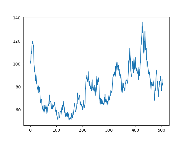
Exercise 9.2.2: Plotting results
Plot your stock path using matplotlib - you will certainly want to google this
Hint Just use plt.plot nothing fancy!
# Solve me!
you should get the following
Exercise 9.2.3: Monte Carlo
In Exercise 9.2.1 you simulated a single path of a stock using GBM. Now create paths_num = 1000 paths and store each of these paths in another list named paths
Hint paths will be a list of lists & you will require two for loops. I have declared the empty list for you to fill below
and to help you on the way I have done the first loop… You will need to finish the code off by adding another loop and the formula for caluclating $s_t$.
Lets restrict this time to one year of simulation to save our CPUs.
import numpy as np

np.random.seed(42)
sigma = .6729                           # annualised volatility of 67.29%
dt = 1/252                              # using annualised vol so need days as frac of yr
r = 0.02                                # annualised expected return
path_len = 252                          # only simulating 1y this time

paths_n = 1000
paths = []
for i in range(paths_n):
    s_t = 100
    path = [s_t]
    ...
    # solve me!
(The full solution takes about 3-4seconds to run on my macbook) TO verify your solution you should get
>>> paths[3][:5]
[100,
 104.481881330148,
 100.2784519513296,
 112.02421958412168,
 114.29778249864029]
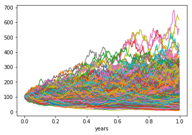
Exercise 9.2.4: Plotting multiple lines on one plot
Plot all 1000 paths with pandas using dt as the index. This is a little more involved so read carefully!
When we created paths we created an object like
[
    [ s_00, s_01, ... , s_0n],  # indexed by paths[0]
    [ s_10, s_11, ... , s_1n],  # indexed by paths[1]
    [ ... , ... , ... , ... ],
    [ s_m0, s_m1, ... , s_mn]   # indexed by paths[m]
] #   ^paths[m][0]      ^paths[m][n]
This makes the zeroth axis the path index and the first axis the time index. However, in pandas and plotting in matplotlib we generally store the time index as the zeroth index and the path index as the first index.
To store in pandas we need to transpose (swap round the referencing) so that in the above example we would change paths[m][n] -> paths[n][m]. This is the same as transposing in Excel.
You can do this with a few different options
paths_df = pd.DataFrame(paths).Tpaths_df = pd.DataFrame(list(zip(*paths)))paths_df = pd.DataFrame(np.array(paths).T)
For sanity would should also probably make the index match the timesteps we are using. Lets create a proper index.
import pandas as pd
import numpy as np
index = pd.Index(np.arange(path_len) * dt, name='years')
Now create the DataFrame with this index. Google if you get stuck.
paths_df = pd.DataFrame(paths, columns=index).T
Make sure that you can pass this test! If you can’t think about the order in which you created the index and then transposed the DataFrame
assert all(paths_df.index.values == index.values)
Now plot with the default pandas plot function. Make sure to pass the argument legend=None!
# Solve me!
you should get the following
Exercise 9.2.5: Prove empirically GBM returns are Normally distributed
Prove that the 1-step stock returns are normally distributed under the GBM model by fitting a Gaussian distribution to the probability distribution function of the 1-day returns - Don’t worry it’s not as hard as it sounds :)
Exercise 9.2.5.1: Calculate 1-day returns using a pandas object
You will need to calculate 1-day returns. You have two options for this:
- Absolute returns $\frac{s_{t} - s_{t-1}}{s_{t-1}}$
- Log returns $\ln s_{t} - \ln s_{t-1}$
Without proof 2 is equal to 1 if $\Delta t \ll T$
e.g. if using years you want to be using a unit of $\Delta t$ that is roughly 100th of a year or smaller
Hint there are four things that might help in googling: "pandas diff", numpy natural log, "pandas shift", "pandas dropna" also remember Google !!
rets_1d = ...
# Solve me!
You should get the following as a check
>>> rets_1d.iloc[:3, :2]
                 0         1
years
0.003968  0.020236  0.038088
0.007937 -0.006680  0.089136
0.011905  0.026636  0.042946
Exercise 9.2.5.3: Check your results
This isn’t so much of an exercise but simply a check for the previous exercise to ensure you have it correct! The maths isn’t too important. If you like, you can ignore it all and just run the code below. You should expect differences less than 1% if you have it correct
Without proof (see here for one) we state that the n-day returns, $R_n$ follow a Normal distribution
\[R_n \sim \mathcal{N}(\mu_n, \sigma_n)\]where
\(\mu_n = \left(r_T - \frac{1}{2}\sigma_T^2\right)n\Delta t\) \(\sigma_n = \sigma_T \sqrt{n\Delta t}\)
such that for T=252 (i.e. a year in our model) $r_T$ is the annualised rate of return (drift) and similarly $\sigma_T$ is the annualised volatility.
Lets take as a fact that we can model a probability distribution function (how likely an event) by using scipy.stats.norm.fit. Then the following snippet of code will confirm your results with theory as a check
# rets_1d should be your result from previous ... you should be able to run it to get the below
import scipy.stats
mean_th = (r - .5*sigma**2)*dt
stdv_th = sigma * np.sqrt(dt)

mean_ac, stdv_ac = scipy.stats.norm.fit(rets_1d)
print(f'Difference in mean samples vs theory: {100*(mean_th - mean_ac)/mean_ac:5.2f}%')
print(f'Difference in stdv samples vs theory: {100*(stdv_th - stdv_ac)/stdv_ac:5.2f}%')
Note Google f-string formatting!
After running the code about you should get the following the show that you have converged to the mean and standard deviation of a normal distribution
Difference in mean samples vs theory:  0.99%
Difference in stdv samples vs theory: -0.01%
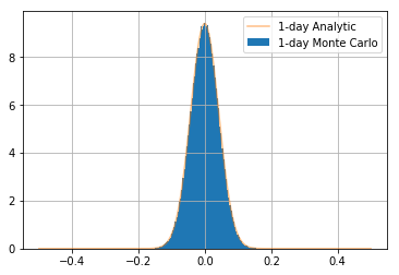
Exercise 9.2.5.3: Plot theory vs. empirical results (reusing matplotlib axes)
This exercise isn’t so much an exercise rather than an example of how to resuse a matplotlib axis object to draw another line.
Compare this with the theory visually by plotting the theoretical distribution and showing its equivalence with the following code
import scipy.stats

# you can access the numpy array beneath the pandas object by .values - then everything is numpy again
rets_1d_all_paths = rets_1d.values.ravel() # get the returns from every path for more samples (google ravel)
x = np.linspace(-.5, .5, 200)              # an array of 200 numbers equally spaced between -.5 and .5

# note that you can chain "." methods in ()
# because recall that unless you have (item,) it doesn't create a tuple!
ax = (
    pd.Series(rets_1d_all_paths) # convert back to pd.Series to use .hist()
    .hist(bins=100, density=True, label='1-day Monte Carlo')
)

# use the same axis object that was returned from .hist()
theory = scipy.stats.norm.pdf(x, mean_th, stdv_th)
ax.plot(x, theory, alpha=0.5, label='1-day Analytic')
ax.legend()
you should get the following
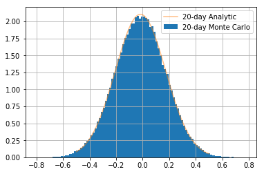
[Optional: This requires undergrad maths!] Exercise 9.2.5.4: Show this holds for 20-day returns
Show the same is true for 20day returns by plotting the relationship with 20-day returns
Note that this exercise is really aimed at structurers, derivatives traders and quants - if you haven’t studied stochastic calculus at university then just ignore this question or ask a quant if you find it interesting
# Solve me!
you should get the following