Contents
This is a beginners introduction. Each topic, subtopic and even sentence most likely has alternatives and improvements in modern literature. If a topic interests you hit you favourite search engine and you will find a lot more information.
Expected background
- Programming The level of programming expected is beginner. You should be comfortable with lists, data structures, iteration and be familiar with numpy.
- Maths The level of maths is GCSE/AS level (upper-high school). You should be able to taken derivatives of exponential functions and be familiar with the chain-rule.
Theory
The XOR function
The XOR function is the simplest (afaik) non-linear function. Is is impossible to separate True results from the False results using a linear function.
def xor(x1, x2):
    """returns XOR"""
    return bool(x1) != bool(x2)

x = np.array([[0,0],[0,1],[1,0],[1,1]])
y = np.array([xor(*x) for x in inputs])
This is clear on a plot
import pandas as pd
import seaborn as sns
sns.set()

data = pd.DataFrame(x, columns=['x1', 'x2'])
data['xor'] = y
sns.scatterplot(data=data, x='x1', y='x2', style='xor', hue='xor', s=100)
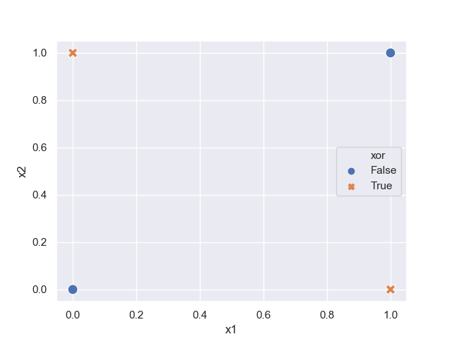
A neural network is essentially a series of hyperplanes (a plane in N dimensions) that group / separate regions in the target hyperplane.
Two lines is all it would take to separate the True values from the False values in the XOR gate.
The Perceptron
There’s lots of good articles about perceptrons. To quickly summarise, a perceptron is essentially a method of separating a manifold with a hyperplane. This is just drawing a straight line to separate an n-dimensional space into two regions: True or False. I will interchangeably refer to these as neurons or perceptrons. Arguablly different, they are basically the same thing.
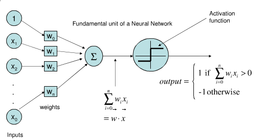
Activation functions
The way our brains work is like a sort of step function. Neurons fires a 1 if there is enough build up of voltage else it doesn’t fire (i.e a zero). We aim, via the percepton, to recreate this behaviour.
The problem with a step function is that they are discontinuous. This creates problems with the practicality of the mathematics (talk to any derivatives trader about the problems in hedging barrier options at the money). Thus we tend to use a smooth functions, the sigmoid, which is infinitely differentiable, allowing us to easily do calculus with our model.
def sigmoid(x):
    return 1/(1 + np.exp(-x))
Hyperplanes
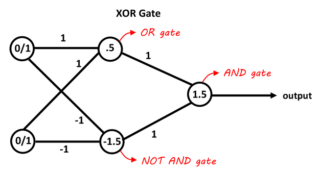
A single perceptron, therefore, cannot separate our XOR gate because it can only draw one straight line.
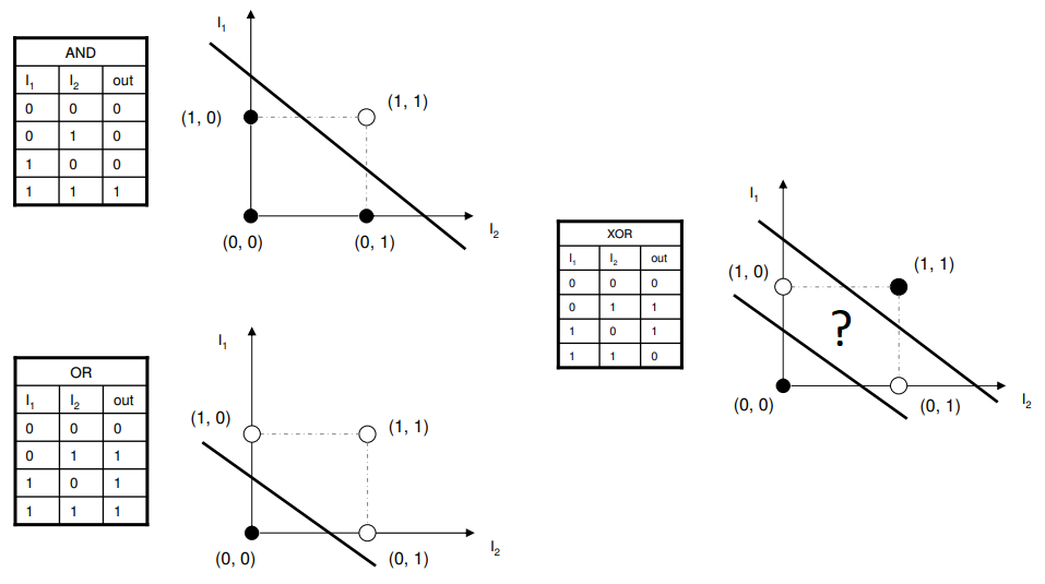
The trick is to realise that we can just logically stack two perceptrons. Two perceptrons that will draw straight lines, and another perceptron that serves to combine these two separate signals into a single signal that just has to differntiate between a single True / False boundary.
Learning parameters
The “knowledge” of a neural network is all contained in the learned parameters which are the weights and bias. The weights are multiplied to each signal sent by their respective perceptrons and the bias are added as $y(x) = wx + b$ where $w$ is the weight and $b$ is the bias.
The backpropagation algorithm (backprop.) is the key method by which we seqeuntially adjust the weights by backpropagating the errors from the final output neuron.
We define define the error as anything that will decrease as we approach the target distribution. Let $E$ be the error function given by
\[E = \frac{1}{2}(y - y_{o})^2\]where $y_o$ is the result of the output layer (the prediction) and $y$ is the true value given in the training data.
Later we will require the derivative of this function so we can add in a factor of 0.5 which simplifies the derivative.
def error(target, prediction):
    return .5 * (target - prediction)**2
| *Note: Explicitly we should define as the norm like, $E = \frac{1}{2} | y - y_{o} | ^2$ since $y$ and $y_{o}$ are vectors but practically it makes no difference and so I prefer to keep it simple for this tutorial.* |
Algorithm
The learning algorithm consists of the following steps:
- Randomly initialise bias and weights
- Iterate the training data
- Forward propagate: Calculate the neural net the output
- Compute a “loss function”
- Backwards propagate: Calculate the gradients with respect to the weights and bias
- Adjust weights and bias by gradient descent
- Exit when error is minimised to some criteria
Note that here we are trying to replicate the exact functional form of the input data. This is not probabilistic data so we do not need a train / validation / test split as overtraining here is actually the aim.
Back propagation
We want to find the minimum loss given a set of parameters (the weights and biases). Recalling some AS level maths, we can find the minima of a function by minimising the gradient (each minima has zero gradient). Also luckily for us, this problem has no local minima so we don’t need to do any funny business to guarantee convergence.
Real world problems require stochastic gradient descents which “jump about” as they descend giving them the ability to find the global minima given a long enough time.
We therefore have several quantitites that require calculation
$\frac{\partial E}{\partial w_{o}}$,
$\frac{\partial E}{\partial w_{h}}$,
$\frac{\partial E}{\partial b_{o}}$
and $\frac{\partial E}{\partial w_{h}}$ where $h$ and $o$ denote hidden and output layers and $E$ is the total error given by
\[\frac{1}{2}(y - y_{o})^2\]Output layer gradient
Starting at the output layer, and by chain rule,
\[\frac{\partial E}{\partial w_{o}} = \frac{\partial E}{\partial y_{o}} \frac{\partial y_o}{\partial a_{o}} \frac{\partial a_o}{\partial w_{o}}\]This is true because the output layer $y_o = \sigma(a_o)$ varies with respect to the activation $a_o = w_o \cdot y_h + b_o$ in the output layer. The activation in the output layer varies with respect to the weights of the output layer. Recall that this is a partial derivative so we hold the bias of the output layer and the hidden layer output as constants. We can calculate all these terms.
The derivative of the Error with respect to the output layer is just
\[\frac{\partial E}{\partial y_{o}} = -(y - y_o)\]due to the sneaky extra half
def error_derivative(target, prediction):
    return - target + prediction
The derivative of the output layer with respect to the sigmoid is
\[\frac{\partial y_o}{\partial a_{o}} = \frac{\partial \sigma(a_o)}{\partial a_o} = \sigma(a_o) (1 - \sigma(a_o)) = y_o (1 - y_o)\]def sigmoid_derivative(sigmoid_result):
return sigmoid_result * (1 - sigmoid_result)
The derivative of the activation function with respect to the weights is
\[\frac{\partial a_o}{\partial w_{o}} = y_h\]which is just the result from the hidden layer.
The same is true for the bias (changing $w_o$ for $b_o$) except
\[\frac{\partial a_o}{\partial b_{o}} = 1\]Hidden layer gradient
For the hidden layer we just keep expanding. Instead of taking $y_h$ as a variable we now treat it as a function that varies with the output of the hidden layer. Thus instead of stopping at $\frac{\partial a_o}{\partial w_o}$ we must continue since $a_o = w_o \cdot y_h + b_o$ is a fuction of $y_h$ which is no longer a constant.
Recall, if we vary $w_h$, $y_h = \sigma(a_h)$ and further, $a_h = w_h \cdot x + b$ where $x$ is the input training data.
Starting at the output layer, and by chain rule,
\[\frac{\partial E}{\partial w_h} = \frac{\partial E}{\partial y_o} \frac{\partial y_o}{\partial a_o} \frac{\partial a_o}{\partial y_h} \frac{\partial y_h}{\partial a_h} \frac{\partial a_h}{\partial w_h}\]the three extra derivatives we need to calculate are
\[\frac{\partial a_o}{\partial y_h} = w_o\]then recall the derivative of the sigmoid from before
\[\frac{\partial y_h}{\partial a_h} = y_h (1 - y_h)\]and finally
\[\frac{\partial a_h}{\partial w_h} = x\]and again the bias are the same except $\frac{\partial a_h}{\partial b_h} = 1$
Parameter updates
Let all the parameters be defined in the vector $\theta = (w_o, w_h, b_o, b_h)$. Then they are all updated like
\[\theta \leftarrow \theta - \alpha \frac{\partial E}{\partial \theta}\]where $\alpha$ is the learning rate that is fixed at some constant (mysteriously, usually about 0.02) and this defines how fast we descend the gradient. Too fast and we overshoot and too small and it takes too long.
Explicitly for $w_o, b_o$ this would be,
\[w_o \leftarrow w_o + \alpha y^T_h \left((y_o - y) y_o (1 - y_o)\right)\\ b_o \leftarrow b_o + \alpha (y_o - y) y_o (1 - y_o)\]where the $y_h^T$ denotes the transpose of the vector $y_h$. I was a bit underhand in the maths to simplify, but as we will see there is some care required with transposing of dot products when multiplying the weights and layers.
Implementation
Initialisation
Initialise the weights and bias like
import numpy as np
def xor(x1, x2):
return bool(x1) != bool(x2)
x = np.array([[0, 0], [0, 1], [1, 0], [1, 1]])
y = np.array([xor(*i) for i in x])
# I explicitly name these for clarity
n_neurons_input, n_neurons_hidden, n_neurons_output = 2, 2, 1
# if this confuses you draw out all the possible wasy to connect the
# first two neurons remembering that we have only connections between layers
# and not between neurons on the same layer
w_hidden = np.random.random(size=(n_neurons_input, n_neurons_hidden))
b_hidden = np.random.random(size=(1, n_neurons_hidden))
w_output = np.random.random(size=(n_neurons_hidden, n_neurons_output))
b_output = np.random.random(size=(1, n_neurons_output))
Forward Propagation
We now have a neural network (albeit a lousey one!) that can be used to make a prediction. To make a prediction we must cross multiply all the weights with the inputs of each respective layer, summing the result and adding bias to the sum.
The action of cross multiplying all combinations of two vectors and summing the result is just the dot product, so that a single forward propagation is given as
def sigmoid(x):
return 1/(1 + np.exp(-x))
y_hidden = sigmoid(np.dot(x, w_hidden) + b_hidden)
y_output = sigmoid(np.dot(y_hidden, w_output) + b_output)
where y_output is now our estimation of the function from the neural network.
Back propagation
The back propagation is then done
def sigmoid_derivative(sigmoid_result):
    return sigmoid_result * (1 - sigmoid_result)
grad_output = (- y + y_output) * sigmoid_derivative(y_output)
grad_hidden = grad_output.dot(w_output.T) * sigmoid_derivative(y_hidden)
The updates require a little explanation of the cheats I did before in the theory section. The function, $a_o = w_o \cdot y_h + b_o$ is actually a vector equation so explicitly, $a_o = y_h^T w_o + b_o$ and similarly, $a_h = x^T w_h + b_h$ which gives some intuition why we need to do the transposes below
w_output -= alpha * y_hidden.T.dot(grad_output)
w_hidden -= alpha * x.T.dot(grad_hidden)
The biases we recall had a derivative of 1. In reality this is the identity, or a vector of 1s so it reduces to a simple sum of all elements in the vector
b_output -= alpha * np.sum(grad_output, axis=0, keepdims=True)
b_hidden -= alpha * np.sum(grad_hidden, axis=0, keepdims=True)
Iteration / Early Stopping
We want to stop after some number of iterations. Therefore in our loop we can do something like below to exit early. We should also store some of the variables and gradients to ensure convergence.
import itertools

errors = []
params = []
grads = []
while True:
    # forward prop

    # calculate mean error of all the errors for this epoch
    e = error(y, y_output).mean()
    if e < 1e-4:
        break

    # back prop

    # update parameters

    # record intermediate results the concatenate just flattens all the
    # matrixes and arrays out into a single "row"
    errors.append(e)
    grads.append(np.concatenate((grad_output.ravel(), grad_hidden.ravel())))
    params.append(np.concatenate((w_output.ravel(), b_output.ravel(),
                                  w_hidden.ravel(), b_hidden.ravel())))
Experiment
Full script
Putting it all together we have
import itertools
import numpy as np

np.random.seed(42) # this makes sure you get the same results as me

def xor(x1, x2):
    return bool(x1) != bool(x2)

def sigmoid(x):
    return 1 / (1 + np.exp(-x))

def sigmoid_derivative(sigmoid_result):
    return sigmoid_result * (1 - sigmoid_result)

def error(target, prediction):
    return .5 * (target - prediction)**2

def error_derivative(target, prediction):
    return - target + prediction

x = np.array([[0, 0], [0, 1], [1, 0], [1, 1]])
y = np.array([[xor(*i)] for i in x], dtype=int)

alpha = 0.02
n_neurons_input, n_neurons_hidden, n_neurons_output = 2, 2, 1

w_hidden = np.random.random(size=(n_neurons_input, n_neurons_hidden))
b_hidden = np.random.random(size=(1, n_neurons_hidden))

w_output = np.random.random(size=(n_neurons_hidden, n_neurons_output))
b_output = np.random.random(size=(1, n_neurons_output))

errors = []
params = []
grads = []
while True:
    # forward prop
    y_hidden = sigmoid(np.dot(x, w_hidden) + b_hidden)
    y_output = sigmoid(np.dot(y_hidden, w_output) + b_output)

    # calculate mean error of all the errors for this epoch
    e = error(y, y_output).mean()
    if e < 1e-4:
        break

    # back prop
    grad_output = error_derivative(y, y_output) * sigmoid_derivative(y_output)
    grad_hidden = grad_output.dot(w_output.T) * sigmoid_derivative(y_hidden)

    # update parameters
    w_output -= alpha * y_hidden.T.dot(grad_output)
    w_hidden -= alpha * x.T.dot(grad_hidden)

    b_output -= alpha * np.sum(grad_output)
    b_hidden -= alpha * np.sum(grad_hidden)

    # record intermediate results
    errors.append(e)
    grads.append(np.concatenate((grad_output.ravel(), grad_hidden.ravel())))
    params.append(np.concatenate((w_output.ravel(), b_output.ravel(),
                                  w_hidden.ravel(), b_hidden.ravel())))
This takes about a minute to run on my macbook. We can now use the model to approximate XOR
>>> def predict(x):
>>>     y_hidden = sigmoid(np.dot(x, w_hidden) + b_hidden)
>>>     return sigmoid(np.dot(y_hidden, w_output) + b_output)
>>> predict(x)
array([[0.01505756],
       [0.98652214],
       [0.98652109],
       [0.01448912]])
As we can see we’re in the order of $10^{-2}$ which makes sense as we minimise the square error to the order of $10^{-4}$.
If this was a real problem, we would save the weights and bias as these define the model.
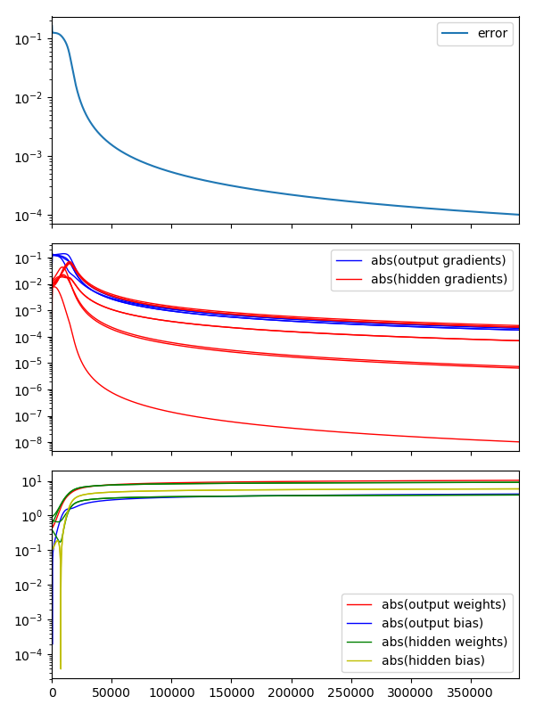
Convergence checks
We should check the convergence for any neural network across the paramters.
The simplest check is the error convergence. We should make sure that the error is decreasing. in larger networks the error can jump around quite erractically so often smoothing (e.g. EWMA) is used to see the decline.
It is also sensible to make sure that the parameters and gradients are cnoverging to sensible values. Furthermore, we would expect the gradients to all approach zero.
It is very important in large networks to address exploding parameters as they are a sign of a bug and can easily be missed to give spurious results.
I use Pandas combined with matplotlib to plot more easily
import matplotlib.pyplot as plt
import pandas as pd

fig, axes = plt.subplots(3, 1, figsize=(6, 8), sharex=True)

pd.DataFrame(errors, columns=['error']).plot(ax=axes[0], logy=True)
df_grads = pd.DataFrame(grads)
df_params = pd.DataFrame(params)

for i in range(4):
    axes[1].plot(df_grads.iloc[:, i].abs(), c='b', label='abs(output gradients)' if i==1 else '__nolabel', lw=1)
for i in range(4, 12):
    axes[1].plot(df_grads.iloc[:, i].abs(), c='r', label='abs(hidden gradients)' if i==4 else '__nolabel', lw=1)

for i in range(1, 2):
    axes[2].plot(df_params.iloc[:, i].abs(), c='r', label='abs(output weights)' if i==1 else '__nolabel', lw=1)

axes[2].plot(df_params.iloc[:, 2].abs(), c='b', label='abs(output bias)', lw=1)

for i in range(3, 7):
    axes[2].plot(df_params.iloc[:, i].abs(), c='g', label='abs(hidden weights)' if i==3 else '__nolabel', lw=1)

for i in range(7, 9):
    axes[2].plot(df_params.iloc[:, i].abs(), c='y', label='abs(hidden bias)' if i==7 else '__nolabel', lw=1)

axes[1].legend()
axes[1].set_yscale('log')

axes[2].legend()
axes[2].set_yscale('log')

fig.tight_layout()
Vanishing gradient problem
It is noticable that the gradient of the hidden layer is considerably smaller than the output layer. This is normal.
In fact it presents a problem. One of the main problems historically with neural networks were that the gradients became too small too quickly as the network grew. In fact so small so quickly that the change in a deep parameter value causes such a small change in the output that it either gets lost in machine noise. Or, in the case of probabilistic models, lost in dataset noise.
This meant that neural networks couldn’t be used for a lot of the problems that required complex network architecture.
There are several workarounds for this problem which largely fall into architecture (e.g. ReLu) or algorithmic adjustments (e.g. greedy layer training).
The sigmoid, is a key offender in the mix. It maps input numbers onto a “small” range of [0, 1]. There are large regions of the input space which are mapped to an extremely small range. In these regions of the input space, even a large change will produce a small change in the output.
This notebook is an excellent example of choosing Relu instead of sigmoid to avoid the vanishing gradient problem.
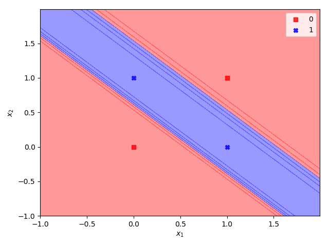
Decision regions
We can plot the hyperplane separation of the decision boundaries. The sigmoid is a smooth function so there is no discontinuous boundary, rather we plot the transition from True into False.
This plot code is a bit more complex than the previous code samples but gives an extremely helpful insight into the workings of the neural network decision process for XOR.
import numpy as np
from matplotlib.colors import ListedColormap
import matplotlib.pyplot as plt

def predict(x):
    y_hidden = sigmoid(np.dot(x, w_hidden) + b_hidden)
    return sigmoid(np.dot(y_hidden, w_output) + b_output)

markers = ('s', 'X')
colors = ('red', 'blue')

x1_min, x1_max = x[:, 0].min() - 1, x[:, 0].max() + 1
x2_min, x2_max = x[:, 1].min() - 1, x[:, 1].max() + 1
xx1, xx2 = np.meshgrid(np.arange(x1_min, x1_max, resolution),
                       np.arange(x2_min, x2_max, resolution))

z = predict(np.array([xx1.ravel(), xx2.ravel()]).T)
z = z.reshape(xx1.shape)

fig, ax = plt.subplots()
ax.contourf(xx1, xx2, z, alpha=0.4, cmap=ListedColormap(colors))
ax.set_xlim(xx1.min(), xx1.max())
ax.set_ylim(xx2.min(), xx2.max())

for idx, cl in enumerate(np.unique(y)):
    ax.scatter(x=x[(y == cl).ravel(), 0],
               y=x[(y == cl).ravel(), 1],
               alpha=0.8, c=colors[idx],
               marker=markers[idx], label=cl)
ax.legend()
ax.set_xlabel('$x_1$')
ax.set_ylabel('$x_2$')
fig.tight_layout()
A converged result should have hyperplanes that separate the True and False values.